Semivariogram exploration#
Rushing into Kriging is a bad idea. You can interpolate values automatically but never know if a process is spatially dependent. The kriging model will return something even when there is no spatial dependency, and it is a dangerous situation because the output might look correct, being wildly wrong.
The easiest way to deal with this problem is to check the variogram before modeling. Feel obligated to do this manual step because it could save you time and money! Variograms will tell you if there is a spatial relation between point pairs and how distance defines it.
In this exercise, we compute the experimental semivariogram, check it, and apply different theoretical models to find the best fit.
Prerequisites#
Domain:
semivariance and covariance functions
Package:
installation
Programming:
Python basics
Table of contents#
Data preparation
Create the experimental variogram
Set manually different semivariogram models
Fit the theoretical model automatically
Export model
Import model
Dataset#
Dataset in this tutorial is the Digital Elevation Model around Gorzów Wielkopolski city in Poland.
[42]:
import geopandas as gpd
import numpy as np
import pandas as pd

import matplotlib.pyplot as plt

from pyinterpolate import reproject_flat, ExperimentalVariogram, build_theoretical_variogram, TheoreticalVariogram
Chapter 1: data preparation#
[43]:
DEM_FILE = '../data/dem.csv'
[44]:
df = pd.read_csv(DEM_FILE)
df.head()
[44]:
| longitude | latitude | dem | |
|---|---|---|---|
| 0 | 15.115241 | 52.765146 | 91.275597 |
| 1 | 15.115241 | 52.742790 | 96.548294 |
| 2 | 15.115241 | 52.710706 | 51.254551 |
| 3 | 15.115241 | 52.708844 | 48.958282 |
| 4 | 15.115241 | 52.671378 | 16.817863 |
Data is stored in EPSG:4326 and has geographic coordinates, it must be reprojected to projected coordinate reference system. Polish area can be projected into EPSG:2180 (metric).
We cannot reproject points easily, first we need to transform longitude and latitude columns into shapely Point() objects, and set CRS, and in the next step we can transform those points into EPSG:2180. Pyinterpolate has function reproject_flat() which takes care of all those steps and returns the same object type as input to it (numpy array or pandas DataFrame).
[45]:
r_df = reproject_flat(
    ds=df,
    in_crs=4326,
    out_crs=2180,
    lon_col='longitude',
    lat_col='latitude'
)
[46]:
r_df.head()
[46]:
| dem | longitude | latitude | |
|---|---|---|---|
| 0 | 91.275597 | 238012.301750 | 551466.805222 |
| 1 | 96.548294 | 237878.001294 | 548982.351111 |
| 2 | 51.254551 | 237685.325393 | 545416.708315 |
| 3 | 48.958282 | 237674.140301 | 545209.671315 |
| 4 | 16.817863 | 237449.254870 | 541045.934750 |
We might transform this DataFrame into GeoDataFrame - mostly for plotting purposes, to see what lies behind this dataset.
[47]:
dem_geometry = gpd.points_from_xy(x=r_df['longitude'], y=r_df['latitude'], crs=2180)
dem = gpd.GeoDataFrame(r_df, geometry=dem_geometry)

dem.plot(column='dem', cmap='gist_earth', alpha=0.6, vmin=0, legend=True);
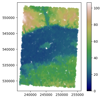
Data covers almost whole area, and this scenario is not realistic, so we will let only 1% of points in a dataset and then proceed to the variogram analysis and modeling.
[48]:
sample = dem.sample(int(0.01 * len(dem)))
sample.plot(column='dem', cmap='gist_earth', alpha=0.6, vmin=0, legend=True);

Chapter 2: Experimental Variogram#
To be sure that we can interpolate missing values with Kriging we must check if there is any relation between observation pairs, and how strong is this relation. We use variograms - plots of the dissimilarity between point pairs along the increasing distance. There are two “types” of variograms that we must be aware of:
The experimental (semi)variogram: directly showing differences between point pairs at specific distances - lags. It could be very messy. We use it to visually check if there is a spatial correlation.
Theoretical (semi)variogram: is a function applied to the experimental variogram. It cannot be any function, there are few of those in literature (and implemented in
pyinterpolate). We can apply those mappings manually or automatically minimizing OLS error between experimental POINTS and theoretical FUNCTION.
We start our analysis by setting up the experimental model. We use class ExperimentalVariogram to set up the object (the class has an alias function build_experimental_variogram() but we won’t use it). Class takes multiple parameters:
values: ArrayLike object with data values.geometries: ArrayLike object with geometries (could be GeoSeries or array with two coordinates in each row).step_size: float - The fixed distance between lags grouping point neighbors.max_range: float - The maximum distance at which the semivariance is calculated.direction: float, optional - Direction of semivariogram, values from 0 to 360 degrees.tolerance: float, optional - Controlling the cone within points are treated as neighbors in directional variogram.custom_bins: numpy array, optional - Custom lags (new in Pyinterpolate 1.x).custom_weights: numpy array, optional - Custom weights assigned to points. Only semivariance values are weighted.is_semivariance: bool, default=True - Calculate experimental semivariance.is_covariance: bool, default=True - Calculate experimental coviariance.as_cloud: bool, default=False - Calculate semivariance point-pairs cloud.
We won’t set direction, tolerance, custom_bins, custom_weights, and as_cloud parameters. Other parameters are set as in the cell below.
[49]:
step_size = 1000  # meters - remember, that this parameter is related to projection!
max_range = 20000  # meters - remember, that this parameter is related to projection!

is_semivariance = True
is_covariance = True

ds = sample[['longitude', 'latitude', 'dem']]
[50]:
experimental_variogram = ExperimentalVariogram(
    values=ds['dem'],
    geometries=ds[['longitude', 'latitude']],
    step_size=step_size,
    max_range=max_range,
    is_semivariance=is_semivariance,
    is_covariance=is_covariance
)
The ExperimentalVariogram object might represent:
semivariance: dissimilarity over a distance, and point cloud semivariances - non-averaged dissimilarities between point pairs,
covariance: similarity over a distance,
variance: non-spatial variance of all points.
The class has two useful methods:
We can print object statistics with the
print()function,We can plot semivariance, covariance, and variance and check how they behave with the
.plot()method.
Let’s check both!
[51]:
print(experimental_variogram)
+---------+--------------------+---------------------+
|   lag   |    semivariance    |      covariance     |
+---------+--------------------+---------------------+
|  1000.0 | 66.71388540855338  |  378.36063443979623 |
|  2000.0 | 130.66628344322854 |  321.7000533191133  |
|  3000.0 | 377.5405401178886  |  150.76532645491605 |
|  4000.0 | 250.66718626708865 |  252.71512355654235 |
|  5000.0 | 325.5561456427749  |  133.18403989988315 |
|  6000.0 | 387.4814906048632  |  30.731695978081564 |
|  7000.0 | 302.07493544556206 |  49.092832725093004 |
|  8000.0 | 469.53885776562294 |  -62.21223171644848 |
|  9000.0 | 486.79931370125183 |  -83.13560908274104 |
| 10000.0 | 512.0646265352149  | -119.11920214846046 |
| 11000.0 |  529.991767276145  |  -76.66066356407669 |
| 12000.0 | 582.4717932210419  |  -80.88872027056644 |
| 13000.0 |  692.506923505966  | -185.99762744031003 |
| 14000.0 | 649.5775483966735  |  -129.2268505373204 |
| 15000.0 | 624.8696046337229  | -151.08544277438932 |
| 16000.0 |  643.74627487684   | -135.27647734328391 |
| 17000.0 | 571.3688648923311  | -127.91473349841077 |
| 18000.0 | 540.0470107890337  | -123.14348266241309 |
| 19000.0 | 600.2575887426275  | -153.57635203377805 |
+---------+--------------------+---------------------+
Lag is a column with the lag center,
semivariance is a column with a dissimilarity metric,
covariance is a column with a similarity metric,
We can plot semivariance and covariance to understand their relation.
[52]:
experimental_variogram.plot(
    semivariance=True,
    covariance=True,
    variance=True
)

Our plot shows three objects:
Circles represent semivariance,
Plus signs represent covariance,
The dashed line is a variance.
We see here that semivariance and covariance are mirrored. What does it mean? It is normal behavior, and we should expect it - semivariance and covariance have symmetrical trends (they differ in a sign). We can read it as:
semivariances show that the dissimilarity between point pairs over a distance increases,
covariances show that the similarity between point pairs over a distance decreases.
In the best-case scenario (data is stationary, e.g., mean and variance don’t change with a distance), variance and covariance should be equal to semivariance.
Chapter 3: Theoretical Variogram#
Manual setting#
We can start modeling theoretical function that optimally describes observed data. Our role is to choose the function type and set three hyperparameters: nugget, sill, and range. You can read more about semivariogram models here: Geostatistics: Theoretical Variogram Models.
Semivariogram has three basic properties:
nugget: the initial value at a zero distance. In most cases, it is zero, but sometimes it represents a bias.
sill: a distance where the semivariogram flattens and reaches approximately 95% of dissimilarity. Sometimes we cannot find a sill; for example, if differences grow exponentially, but in pyinterpolate it is usually set close to the variance of data. In
pyinterpolatewe set partial_sill which is a difference between total sill and nugget.range: is a distance where a variogram reaches its sill. Larger distances are negligible for interpolation.
We are not forced to know all of them at the beginning. The package may easily derive them all with the class TheoriticalVariogram.autofit() method.
We can create a theoretical model in two ways:
Manually, setting model type, nugget, sill, and range.
Semi-automatically, leaving some parameters (from the above) not filled. We will do it in the next chapter.
Models#
We can choose from a set of predefined models:
circular
cubic
exponential
gaussian
linear
power
spherical
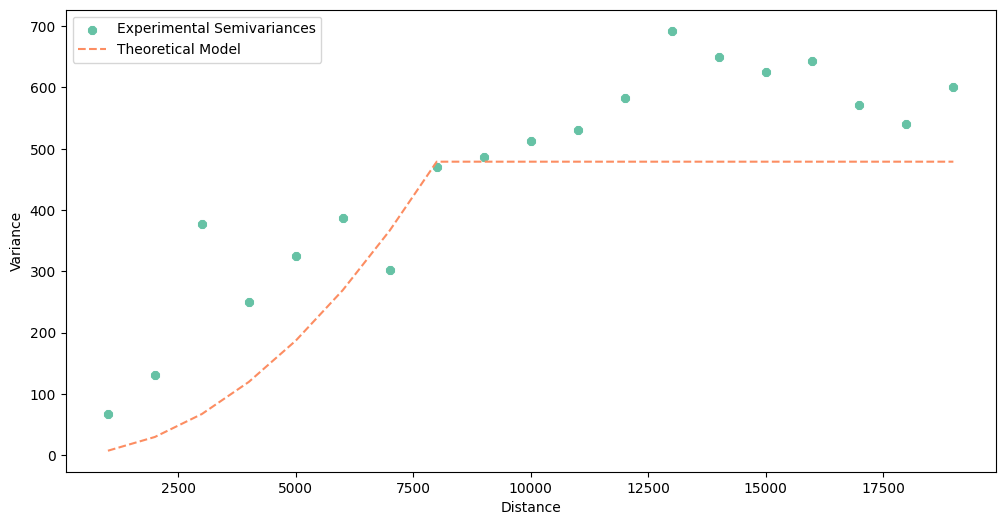
We will set the following:
sill (partial sill) to the experimental variogram variance, (but it might be set to the the last five lags average value of semivariances),
nugget to zero,
range to 8000 (we see in the experimental variogram plot that the semivariance flattens around this range, and it becomes close to the variance).
[53]:
sill = experimental_variogram.variance
nugget = 0
variogram_range = 8000
[54]:
# circular

circular_model = build_theoretical_variogram(experimental_variogram=experimental_variogram,
                                             models_group='circular',
                                             sill=sill,
                                             rang=variogram_range,
                                             nugget=nugget)
[55]:
print(circular_model)
* Selected model: Circular model
* Nugget: 0
* Sill: 478.90567078851103
* Range: 8000
* Spatial Dependency Strength is Undefined: nugget equal to 0, cannot estimate
* Mean Bias: None
* Mean RMSE: 106.4369154595279
* Error-lag weighting method: equal


+---------+--------------------+--------------------+---------------------+
|   lag   |    theoretical     |    experimental    |   bias (real-yhat)  |
+---------+--------------------+--------------------+---------------------+
|  1000.0 | 76.02124683696297  | 66.71388540855338  |  -9.307361428409592 |
|  2000.0 | 150.8372591039797  | 130.66628344322854 | -20.170975660751168 |
|  3000.0 | 223.18223486037513 | 377.5405401178886  |  154.35830525751348 |
|  4000.0 | 291.65249083970144 | 250.66718626708865 |  -40.98530457261279 |
|  5000.0 | 354.58310049417867 | 325.5561456427749  | -29.026954851403787 |
|  6000.0 | 409.8026413531391  | 387.4814906048632  | -22.321150748275898 |
|  7000.0 | 453.9807623558251  | 302.07493544556206 | -151.90582691026304 |
|  8000.0 | 478.90567078851103 | 469.53885776562294 |  -9.366813022888095 |
|  9000.0 | 478.90567078851103 | 486.79931370125183 |  7.893642912740802  |
| 10000.0 | 478.90567078851103 | 512.0646265352149  |  33.15895574670384  |
| 11000.0 | 478.90567078851103 |  529.991767276145  |  51.08609648763394  |
| 12000.0 | 478.90567078851103 | 582.4717932210419  |  103.5661224325309  |
| 13000.0 | 478.90567078851103 |  692.506923505966  |   213.601252717455  |
| 14000.0 | 478.90567078851103 | 649.5775483966735  |  170.67187760816245 |
| 15000.0 | 478.90567078851103 | 624.8696046337229  |  145.9639338452119  |
| 16000.0 | 478.90567078851103 |  643.74627487684   |  164.84060408832892 |
| 17000.0 | 478.90567078851103 | 571.3688648923311  |  92.46319410382006  |
| 18000.0 | 478.90567078851103 | 540.0470107890337  |  61.14134000052269  |
| 19000.0 | 478.90567078851103 | 600.2575887426275  |  121.35191795411646 |
+---------+--------------------+--------------------+---------------------+
[56]:
circular_model.plot()

[57]:
# cubic

cubic_model = build_theoretical_variogram(experimental_variogram=experimental_variogram,
                                          models_group='cubic',
                                          sill=sill,
                                          rang=variogram_range,
                                          nugget=nugget)
[58]:
print(cubic_model)
* Selected model: Cubic model
* Nugget: 0
* Sill: 478.90567078851103
* Range: 8000
* Spatial Dependency Strength is Undefined: nugget equal to 0, cannot estimate
* Mean Bias: None
* Mean RMSE: 112.51542324377124
* Error-lag weighting method: equal


+---------+--------------------+--------------------+---------------------+
|   lag   |    theoretical     |    experimental    |   bias (real-yhat)  |
+---------+--------------------+--------------------+---------------------+
|  1000.0 | 44.24686603199425  | 66.71388540855338  |  22.46701937655913  |
|  2000.0 | 145.66080834697556 | 130.66628344322854 |  -14.99452490374702 |
|  3000.0 | 262.4988714324439  | 377.5405401178886  |  115.04166868544473 |
|  4000.0 | 363.8560662826773  | 250.66718626708865 | -113.18888001558867 |
|  5000.0 | 432.92635147156795 | 325.5561456427749  | -107.37020582879308 |
|  6000.0 | 467.67401160879393 | 387.4814906048632  |  -80.19252100393072 |
|  7000.0 | 478.0522323071066  | 302.07493544556206 | -175.97729686154452 |
|  8000.0 | 478.90567078851103 | 469.53885776562294 |  -9.366813022888095 |
|  9000.0 | 478.90567078851103 | 486.79931370125183 |  7.893642912740802  |
| 10000.0 | 478.90567078851103 | 512.0646265352149  |  33.15895574670384  |
| 11000.0 | 478.90567078851103 |  529.991767276145  |  51.08609648763394  |
| 12000.0 | 478.90567078851103 | 582.4717932210419  |  103.5661224325309  |
| 13000.0 | 478.90567078851103 |  692.506923505966  |   213.601252717455  |
| 14000.0 | 478.90567078851103 | 649.5775483966735  |  170.67187760816245 |
| 15000.0 | 478.90567078851103 | 624.8696046337229  |  145.9639338452119  |
| 16000.0 | 478.90567078851103 |  643.74627487684   |  164.84060408832892 |
| 17000.0 | 478.90567078851103 | 571.3688648923311  |  92.46319410382006  |
| 18000.0 | 478.90567078851103 | 540.0470107890337  |  61.14134000052269  |
| 19000.0 | 478.90567078851103 | 600.2575887426275  |  121.35191795411646 |
+---------+--------------------+--------------------+---------------------+
[59]:
cubic_model.plot()

[60]:
# Exponential model

exponential_model = build_theoretical_variogram(experimental_variogram=experimental_variogram,
                                                models_group='exponential',
                                                sill=sill,
                                                rang=variogram_range,
                                                nugget=nugget)
print(exponential_model)
* Selected model: Exponential model
* Nugget: 0
* Sill: 478.90567078851103
* Range: 8000
* Spatial Dependency Strength is Undefined: nugget equal to 0, cannot estimate
* Mean Bias: None
* Mean RMSE: 172.56017194999464
* Error-lag weighting method: equal


+---------+--------------------+--------------------+--------------------+
|   lag   |    theoretical     |    experimental    |  bias (real-yhat)  |
+---------+--------------------+--------------------+--------------------+
|  1000.0 | 56.27289968745207  | 66.71388540855338  | 10.440985721101313 |
|  2000.0 | 105.93355936108222 | 130.66628344322854 | 24.73272408214632  |
|  3000.0 | 149.7589377033685  | 377.5405401178886  | 227.7816024145201  |
|  4000.0 | 188.4346983450342  | 250.66718626708865 | 62.232487922054446 |
|  5000.0 | 222.56593731640734 | 325.5561456427749  | 102.99020832636754 |
|  6000.0 | 252.68664999001882 | 387.4814906048632  | 134.7948406148444  |
|  7000.0 | 279.26808562812147 | 302.07493544556206 | 22.806849817440593 |
|  8000.0 | 302.72612024499887 | 469.53885776562294 | 166.81273752062407 |
|  9000.0 | 323.42776313511536 | 486.79931370125183 | 163.37155056613648 |
| 10000.0 | 341.6968988640556  | 512.0646265352149  | 170.3677276711593  |
| 11000.0 | 357.81935455774294 |  529.991767276145  | 172.17241271840203 |
| 12000.0 | 372.04737176947935 | 582.4717932210419  | 210.42442145156258 |
| 13000.0 | 384.60355288875706 |  692.506923505966  | 307.90337061720896 |
| 14000.0 | 395.6843438348108  | 649.5775483966735  | 253.89320456186266 |
| 15000.0 | 405.4631075228907  | 624.8696046337229  | 219.40649711083222 |
| 16000.0 | 414.0928361887279  |  643.74627487684   | 229.65343868811203 |
| 17000.0 | 421.7085450064747  | 571.3688648923311  | 149.66031988585638 |
| 18000.0 | 428.4293844491225  | 540.0470107890337  | 111.61762633991123 |
| 19000.0 | 434.3605044400275  | 600.2575887426275  | 165.89708430259998 |
+---------+--------------------+--------------------+--------------------+
[61]:
exponential_model.plot()
[62]:
# Gaussian model
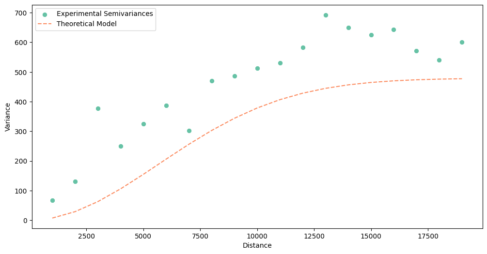
gaussian_model = build_theoretical_variogram(experimental_variogram=experimental_variogram,
models_group='gaussian',
sill=sill,
rang=variogram_range,
nugget=nugget)
print(gaussian_model)
* Selected model: Gaussian model
* Nugget: 0
* Sill: 478.90567078851103
* Range: 8000
* Spatial Dependency Strength is Undefined: nugget equal to 0, cannot estimate
* Mean Bias: None
* Mean RMSE: 159.98897643128805
* Error-lag weighting method: equal


+---------+--------------------+--------------------+--------------------+
|   lag   |    theoretical     |    experimental    |  bias (real-yhat)  |
+---------+--------------------+--------------------+--------------------+
|  1000.0 | 7.424744235536801  | 66.71388540855338  | 59.28914117301658  |
|  2000.0 | 29.015427794333753 | 130.66628344322854 | 101.65085564889478 |
|  3000.0 | 62.825213477796176 | 377.5405401178886  | 314.7153266400924  |
|  4000.0 | 105.93355936108222 | 250.66718626708865 | 144.73362690600644 |
|  5000.0 | 154.86188481421806 | 325.5561456427749  | 170.69426082855682 |
|  6000.0 | 206.03344490697575 | 387.4814906048632  | 181.44804569788747 |
|  7000.0 | 256.19385082954307 | 302.07493544556206 | 45.881084616018995 |
|  8000.0 | 302.72612024499887 | 469.53885776562294 | 166.81273752062407 |
|  9000.0 | 343.8241237029969  | 486.79931370125183 | 142.9751899982549  |
| 10000.0 | 378.52158882000424 | 512.0646265352149  | 133.54303771521063 |
| 11000.0 | 406.6017289289635  |  529.991767276145  | 123.39003834718147 |
| 12000.0 | 428.4293844491225  | 582.4717932210419  | 154.04240877191944 |
| 13000.0 | 444.7517070227298  |  692.506923505966  | 247.7552164832362  |
| 14000.0 |  456.506954502525  | 649.5775483966735  | 193.0705938941485  |
| 15000.0 | 464.6681804730809  | 624.8696046337229  | 160.20142416064203 |
| 16000.0 | 470.13420746058165 |  643.74627487684   | 173.6120674162583  |
| 17000.0 | 473.66799080758676 | 571.3688648923311  | 97.70087408474433  |
| 18000.0 | 475.8743341758106  | 540.0470107890337  | 64.17267661322313  |
| 19000.0 | 477.20524505947054 | 600.2575887426275  | 123.05234368315695 |
+---------+--------------------+--------------------+--------------------+
[63]:
gaussian_model.plot()
[64]:
# Linear model
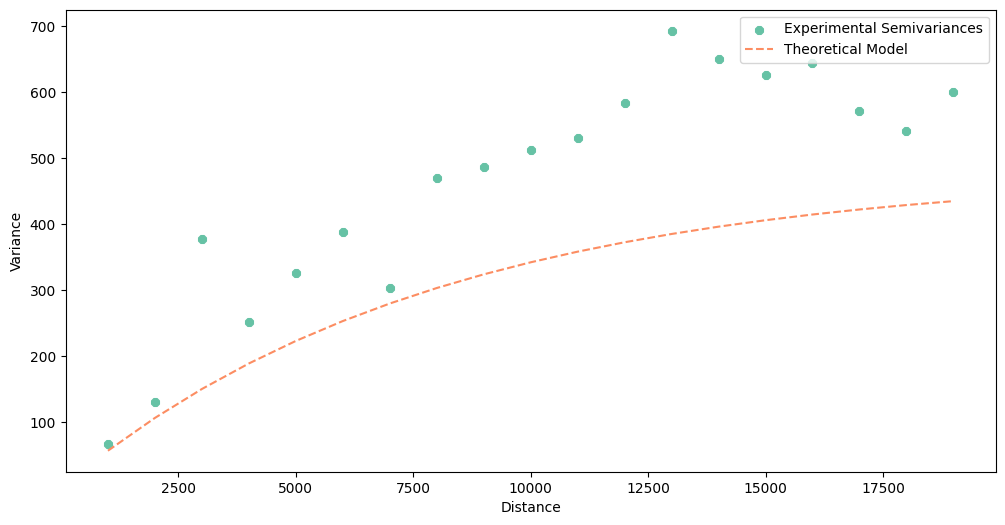
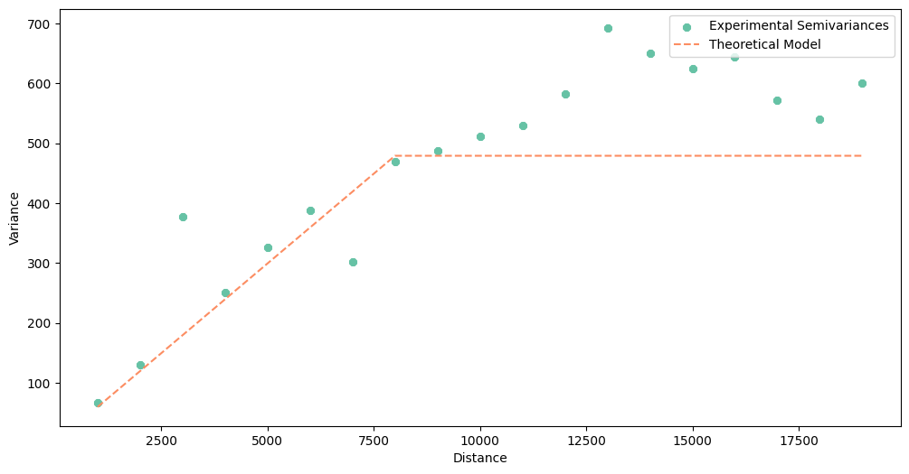
linear_model = build_theoretical_variogram(experimental_variogram=experimental_variogram,
models_group='linear',
sill=sill,
rang=variogram_range,
nugget=nugget)
print(linear_model)
* Selected model: Linear model
* Nugget: 0
* Sill: 478.90567078851103
* Range: 8000
* Spatial Dependency Strength is Undefined: nugget equal to 0, cannot estimate
* Mean Bias: None
* Mean RMSE: 107.47814162764915
* Error-lag weighting method: equal


+---------+--------------------+--------------------+---------------------+
|   lag   |    theoretical     |    experimental    |   bias (real-yhat)  |
+---------+--------------------+--------------------+---------------------+
|  1000.0 | 59.86320884856388  | 66.71388540855338  |  6.850676559989502  |
|  2000.0 | 119.72641769712776 | 130.66628344322854 |  10.939865746100779 |
|  3000.0 | 179.58962654569163 | 377.5405401178886  |  197.95091357219698 |
|  4000.0 | 239.45283539425552 | 250.66718626708865 |  11.214350872833137 |
|  5000.0 | 299.3160442428194  | 325.5561456427749  |  26.240101399955506 |
|  6000.0 | 359.17925309138326 | 387.4814906048632  |  28.30223751347995  |
|  7000.0 | 419.04246193994715 | 302.07493544556206 | -116.96752649438508 |
|  8000.0 | 478.90567078851103 | 469.53885776562294 |  -9.366813022888095 |
|  9000.0 | 478.90567078851103 | 486.79931370125183 |  7.893642912740802  |
| 10000.0 | 478.90567078851103 | 512.0646265352149  |  33.15895574670384  |
| 11000.0 | 478.90567078851103 |  529.991767276145  |  51.08609648763394  |
| 12000.0 | 478.90567078851103 | 582.4717932210419  |  103.5661224325309  |
| 13000.0 | 478.90567078851103 |  692.506923505966  |   213.601252717455  |
| 14000.0 | 478.90567078851103 | 649.5775483966735  |  170.67187760816245 |
| 15000.0 | 478.90567078851103 | 624.8696046337229  |  145.9639338452119  |
| 16000.0 | 478.90567078851103 |  643.74627487684   |  164.84060408832892 |
| 17000.0 | 478.90567078851103 | 571.3688648923311  |  92.46319410382006  |
| 18000.0 | 478.90567078851103 | 540.0470107890337  |  61.14134000052269  |
| 19000.0 | 478.90567078851103 | 600.2575887426275  |  121.35191795411646 |
+---------+--------------------+--------------------+---------------------+
[65]:
linear_model.plot()
[66]:
# Power model

power_model = build_theoretical_variogram(experimental_variogram=experimental_variogram,
                                          models_group='power',
                                          sill=sill,
                                          rang=variogram_range,
                                          nugget=nugget)
print(power_model)
* Selected model: Power model
* Nugget: 0
* Sill: 478.90567078851103
* Range: 8000
* Spatial Dependency Strength is Undefined: nugget equal to 0, cannot estimate
* Mean Bias: None
* Mean RMSE: 131.6193788004333
* Error-lag weighting method: equal


+---------+--------------------+--------------------+--------------------+
|   lag   |    theoretical     |    experimental    |  bias (real-yhat)  |
+---------+--------------------+--------------------+--------------------+
|  1000.0 | 7.482901106070485  | 66.71388540855338  | 59.230984302482895 |
|  2000.0 | 29.93160442428194  | 130.66628344322854 | 100.7346790189466  |
|  3000.0 | 67.34610995463436  | 377.5405401178886  | 310.19443016325425 |
|  4000.0 | 119.72641769712776 | 250.66718626708865 | 130.94076856996088 |
|  5000.0 | 187.07252765176213 | 325.5561456427749  | 138.48361799101275 |
|  6000.0 | 269.38443981853743 | 387.4814906048632  | 118.09705078632578 |
|  7000.0 | 366.66215419745373 | 302.07493544556206 | -64.58721875189167 |
|  8000.0 | 478.90567078851103 | 469.53885776562294 | -9.366813022888095 |
|  9000.0 | 478.90567078851103 | 486.79931370125183 | 7.893642912740802  |
| 10000.0 | 478.90567078851103 | 512.0646265352149  | 33.15895574670384  |
| 11000.0 | 478.90567078851103 |  529.991767276145  | 51.08609648763394  |
| 12000.0 | 478.90567078851103 | 582.4717932210419  | 103.5661224325309  |
| 13000.0 | 478.90567078851103 |  692.506923505966  |  213.601252717455  |
| 14000.0 | 478.90567078851103 | 649.5775483966735  | 170.67187760816245 |
| 15000.0 | 478.90567078851103 | 624.8696046337229  | 145.9639338452119  |
| 16000.0 | 478.90567078851103 |  643.74627487684   | 164.84060408832892 |
| 17000.0 | 478.90567078851103 | 571.3688648923311  | 92.46319410382006  |
| 18000.0 | 478.90567078851103 | 540.0470107890337  | 61.14134000052269  |
| 19000.0 | 478.90567078851103 | 600.2575887426275  | 121.35191795411646 |
+---------+--------------------+--------------------+--------------------+
[67]:
power_model.plot()
[68]:
# Spherical model

spherical_model = build_theoretical_variogram(experimental_variogram=experimental_variogram,
                                              models_group='spherical',
                                              sill=sill,
                                              rang=variogram_range,
                                              nugget=nugget)

print(spherical_model)
* Selected model: Spherical model
* Nugget: 0
* Sill: 478.90567078851103
* Range: 8000
* Spatial Dependency Strength is Undefined: nugget equal to 0, cannot estimate
* Mean Bias: None
* Mean RMSE: 108.209074255922
* Error-lag weighting method: equal


+---------+--------------------+--------------------+---------------------+
|   lag   |    theoretical     |    experimental    |   bias (real-yhat)  |
+---------+--------------------+--------------------+---------------------+
|  1000.0 | 89.32713195371642  | 66.71388540855338  | -22.613246545163037 |
|  2000.0 | 175.8481759926564  | 130.66628344322854 |  -45.18189254942786 |
|  3000.0 | 256.7570442020435  | 377.5405401178886  |  120.7834959158451  |
|  4000.0 | 329.2476486671013  | 250.66718626708865 |  -78.58046240001266 |
|  5000.0 | 390.5139014730534  | 325.5561456427749  |  -64.95775583027853 |
|  6000.0 | 437.7497147051234  | 387.4814906048632  |  -50.26822410026017 |
|  7000.0 | 468.1490004485347  | 302.07493544556206 | -166.07406500297265 |
|  8000.0 | 478.90567078851103 | 469.53885776562294 |  -9.366813022888095 |
|  9000.0 | 478.90567078851103 | 486.79931370125183 |  7.893642912740802  |
| 10000.0 | 478.90567078851103 | 512.0646265352149  |  33.15895574670384  |
| 11000.0 | 478.90567078851103 |  529.991767276145  |  51.08609648763394  |
| 12000.0 | 478.90567078851103 | 582.4717932210419  |  103.5661224325309  |
| 13000.0 | 478.90567078851103 |  692.506923505966  |   213.601252717455  |
| 14000.0 | 478.90567078851103 | 649.5775483966735  |  170.67187760816245 |
| 15000.0 | 478.90567078851103 | 624.8696046337229  |  145.9639338452119  |
| 16000.0 | 478.90567078851103 |  643.74627487684   |  164.84060408832892 |
| 17000.0 | 478.90567078851103 | 571.3688648923311  |  92.46319410382006  |
| 18000.0 | 478.90567078851103 | 540.0470107890337  |  61.14134000052269  |
| 19000.0 | 478.90567078851103 | 600.2575887426275  |  121.35191795411646 |
+---------+--------------------+--------------------+---------------------+
[69]:
spherical_model.plot()
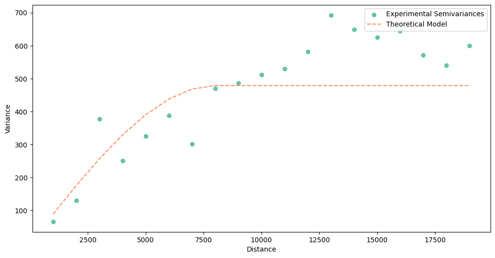
A quick look into Root Mean Squared Errors (RMSE), and we can bet that the best model is linear. We can check each table printed with the print() manually, but instead, we will automatically select model with the lowest RMSE to be sure that we have chosen the best function.
[70]:
models = [
    circular_model, cubic_model, exponential_model, gaussian_model, linear_model, power_model, spherical_model
]

lowest_rmse = np.inf
chosen_model = ''

for _model in models:

    # Get attrs
    model_name = _model.name
    model_rmse = _model.rmse

    # Check error
    if model_rmse < lowest_rmse:
        lowest_rmse = model_rmse
        chosen_model = model_name

    # Print status
    msg = f'Model: {model_name}, RMSE: {model_rmse}'
    print(msg)

msg = f'\nThe best model is {chosen_model} with RMSE {lowest_rmse}'
print(msg)
Model: circular, RMSE: 106.4369154595279
Model: cubic, RMSE: 112.51542324377124
Model: exponential, RMSE: 172.56017194999464
Model: gaussian, RMSE: 159.98897643128805
Model: linear, RMSE: 107.47814162764915
Model: power, RMSE: 131.6193788004333
Model: spherical, RMSE: 108.209074255922

The best model is circular with RMSE 106.4369154595279
Chapter 4: Fit semivariogram model automatically#
We may find the optimal semivariogram model automatically, leaving parameters empty in build_variogram_model() function. This function creates the instance of TheoreticalVariogram object, and calls .autofit() method.
The build_variogram_model() function takes multiple parameters. The most important for us are:
experimental_variogram- the experimental variogram object (ExperimentalVariogramtype)models_group- it could be a single model name, list with multiple model types, or special text aliases to test group of models. By default, this parameter is set tosafe- it compares a list of safe variogram functions that are rather resistant to overfitting. The full list of available options:'all'- the same as list with all models, -'safe'- [‘linear’, ‘power’, ‘spherical’] - as a list: multiple model types to test - as a single model type from: -'circular'-'cubic'-'exponential'-'gaussian'-'linear'-'power'-'spherical'
nugget- nugget (bias) of a variogram. If given, then the nugget is fixed to this valuemin_nugget- default = 0.0 - the minimal fraction of the nugget at a distance 0 to search for the optimal nuggetmax_nugget- default = 0.5 - the maximum fraction of the nugget at a distance 0 to search for the optimal nuggetnumber_of_nuggets- default = 16 - how many equally spaced steps betweenmin_nuggetandmax_nuggetto checkrang- if given, then the range is fixed to this valuemin_range- default = 0.1 - the minimal fraction of a variogram range,0 < min_range <= max_rangemax_range- default = 0.5 - the maximum fraction of a variogram range,min_range <= max_range <= 1. Parametermax_rangegreater than 0.5 raises warningnumber_of_ranges- default = 16 - how many equally spaced ranges are tested betweenmin_rangeandmax_range.sill- if given, it is fixed to this valuemin_sill- default = 0 - the minimal fraction of the variogram variance at lag 0 to find a sill,0 <= min_sill <= max_sillmax_sill- default = 1 - the maximum fraction of the variogram variance at lag 0 to find a sill. It should be lower or equal to 1. It is possible to set it above 1, but then warning is printednumber_of_sills- default = 16 - how many equally spaced sill values are tested betweenmin_sillandmax_sillerror_estimator- default ='rmse'- Error estimation to choose the best model. Available options are:rmse: Root Mean Squared Errormae: Mean Absolute Errorbias: Forecast Biassmape: Symmetric Mean Absolute Percentage Error
In the first run, we will set nugget, sill, and range as fixed values, and we will see which model type (name) algorithm chooses from the all possible models.
[71]:
fitted = build_theoretical_variogram(
    experimental_variogram=experimental_variogram,
    models_group='all',
    nugget=0,
    rang=variogram_range,
    sill=sill
)
[72]:
print(fitted)
* Selected model: Circular model
* Nugget: 0
* Sill: 478.90567078851103
* Range: 8000
* Spatial Dependency Strength is Undefined: nugget equal to 0, cannot estimate
* Mean Bias: None
* Mean RMSE: 106.4369154595279
* Error-lag weighting method: equal


+---------+--------------------+--------------------+---------------------+
|   lag   |    theoretical     |    experimental    |   bias (real-yhat)  |
+---------+--------------------+--------------------+---------------------+
|  1000.0 | 76.02124683696297  | 66.71388540855338  |  -9.307361428409592 |
|  2000.0 | 150.8372591039797  | 130.66628344322854 | -20.170975660751168 |
|  3000.0 | 223.18223486037513 | 377.5405401178886  |  154.35830525751348 |
|  4000.0 | 291.65249083970144 | 250.66718626708865 |  -40.98530457261279 |
|  5000.0 | 354.58310049417867 | 325.5561456427749  | -29.026954851403787 |
|  6000.0 | 409.8026413531391  | 387.4814906048632  | -22.321150748275898 |
|  7000.0 | 453.9807623558251  | 302.07493544556206 | -151.90582691026304 |
|  8000.0 | 478.90567078851103 | 469.53885776562294 |  -9.366813022888095 |
|  9000.0 | 478.90567078851103 | 486.79931370125183 |  7.893642912740802  |
| 10000.0 | 478.90567078851103 | 512.0646265352149  |  33.15895574670384  |
| 11000.0 | 478.90567078851103 |  529.991767276145  |  51.08609648763394  |
| 12000.0 | 478.90567078851103 | 582.4717932210419  |  103.5661224325309  |
| 13000.0 | 478.90567078851103 |  692.506923505966  |   213.601252717455  |
| 14000.0 | 478.90567078851103 | 649.5775483966735  |  170.67187760816245 |
| 15000.0 | 478.90567078851103 | 624.8696046337229  |  145.9639338452119  |
| 16000.0 | 478.90567078851103 |  643.74627487684   |  164.84060408832892 |
| 17000.0 | 478.90567078851103 | 571.3688648923311  |  92.46319410382006  |
| 18000.0 | 478.90567078851103 | 540.0470107890337  |  61.14134000052269  |
| 19000.0 | 478.90567078851103 | 600.2575887426275  |  121.35191795411646 |
+---------+--------------------+--------------------+---------------------+
The chosen model is (most likely) linear, automatically set as the class parameter. The algorithm performs the same steps as we did before. It has selected a model based on the RMSE. All other parameters were untouched.
Now, we let the algorithm find the optimal parameters (model type, nugget, sill, range).
[73]:
fitted = build_theoretical_variogram(experimental_variogram=experimental_variogram)
[74]:
print(fitted)
* Selected model: Spherical model
* Nugget: 24.46175798313624
* Sill: 596.0578687869111
* Range: 14980.760125261822
* Spatial Dependency Strength is strong
* Mean Bias: None
* Mean RMSE: 58.37586447036475
* Error-lag weighting method: equal


+---------+--------------------+--------------------+---------------------+
|   lag   |    theoretical     |    experimental    |   bias (real-yhat)  |
+---------+--------------------+--------------------+---------------------+
|  1000.0 | 84.05545137223926  | 66.71388540855338  |  -17.34156596368588 |
|  2000.0 | 143.11727153379871 | 130.66628344322854 | -12.450988090570178 |
|  3000.0 | 201.1153452402711  | 377.5405401178886  |  176.4251948776175  |
|  4000.0 | 257.5177992641128  | 250.66718626708865 |  -6.850612997024143 |
|  5000.0 | 311.7927603777803  | 325.5561456427749  |  13.763385264994554 |
|  6000.0 | 363.40835535373014 | 387.4814906048632  |  24.073135251133067 |
|  7000.0 | 411.83271096441854 | 302.07493544556206 | -109.75777551885648 |
|  8000.0 | 456.53395398230225 | 469.53885776562294 |  13.004903783320685 |
|  9000.0 | 496.98021117983745 | 486.79931370125183 |  -10.18089747858562 |
| 10000.0 | 532.6396093294809  | 512.0646265352149  |  -20.57498279426602 |
| 11000.0 | 562.9802752036886  |  529.991767276145  |  -32.98850792754365 |
| 12000.0 | 587.4703355749175  | 582.4717932210419  |  -4.998542353875564 |
| 13000.0 | 605.5779172156238  |  692.506923505966  |  86.92900629034227  |
| 14000.0 | 616.7711468982636  | 649.5775483966735  |  32.806401498409855 |
| 15000.0 | 620.5196267700474  | 624.8696046337229  |  4.349977863675576  |
| 16000.0 | 620.5196267700474  |  643.74627487684   |  23.226648106792595 |
| 17000.0 | 620.5196267700474  | 571.3688648923311  |  -49.15076187771626 |
| 18000.0 | 620.5196267700474  | 540.0470107890337  |  -80.47261598101363 |
| 19000.0 | 620.5196267700474  | 600.2575887426275  | -20.262038027419862 |
+---------+--------------------+--------------------+---------------------+
As you see, the model is better, but parameters are different than we have set. Still, the best model is linear. Let’s compare both those models on a single plot.
[75]:
_lags = experimental_variogram.lags
_experimental = experimental_variogram.semivariances
_linear_manual = linear_model.yhat
_automatic = fitted.yhat

plt.figure(figsize=(20, 8))
plt.scatter(_lags, _experimental, color='#762a83')  # Experimental
plt.plot(_lags, _linear_manual, ':p', color='#e7d4e8', mec='black')
plt.plot(_lags, _automatic, ':o', color='#1b7837', mec='black')

plt.title('Comparison of theoretical semivariance models')
plt.legend(['Experimental Semivariances',
            'Manual - ' + linear_model.name,
            'Automatic - ' + fitted.name])
plt.xlabel('Distance')
plt.ylabel('Semivariance')
plt.show()

Chapter 5: Exporting model#
Models could be exported and used for other purposes. It is vital for the semivariogram regularization. Those calculations are computationally intensive, and in production, it is not a good idea to regularize semivariogram every time when you run the Poisson Kriging pipeline. Moreover, theoretical model parameters should be traced and stored for reproducibility and explainability purposes.
Model can be exported to dict with .to_dict() method or to json with .to_json() methods.
[76]:
dict_representation = fitted.to_dict()
[77]:
dict_representation
[77]:
{'experimental_variogram': None,
 'nugget': 24.46175798313624,
 'sill': 596.0578687869111,
 'rang': 14980.760125261822,
 'variogram_model_type': 'spherical',
 'direction': None,
 'spatial_dependence': None,
 'spatial_index': None,
 'yhat': None,
 'errors': None}
[78]:
# Save to json

fitted.to_json('fitted.json')
Chapter 6: Importing fitted model#
We can import a semivariogram model into a TheoreticalVariogram class instance without passing the experimental semivariogram or actual data points. It is helpful for some applications focused on kriging, where we are sure that our semivariogram model fits data well.
We can import a model with two methods .from_dict() if we have our model parameters in the Python dictionary or .from_json() if model parameters are stored in a flat file:
[79]:
model_from_dict = TheoreticalVariogram()
model_from_dict.from_dict(dict_representation)
[80]:
print(model_from_dict)
* Selected model: Spherical model
* Nugget: 24.46175798313624
* Sill: 596.0578687869111
* Range: 14980.760125261822
* Spatial Dependency Strength is strong
* Mean Bias: 0.0
* Mean RMSE: 0.0
* Error-lag weighting method: None
[81]:
model_from_json = TheoreticalVariogram()
model_from_json.from_json('fitted.json')
[82]:
print(model_from_json)
* Selected model: Spherical model
* Nugget: 24.46175798313624
* Sill: 596.0578687869111
* Range: 14980.760125261822
* Spatial Dependency Strength is strong
* Mean Bias: 0.0
* Mean RMSE: 0.0
* Error-lag weighting method: None
That’s all, well done!
Changelog#
Date |
Changes |
Author |
|---|---|---|
2025-11-07 |
Used values and geometries parameters instead of ds in the experimental variogram initialization |
@SimonMolinsky (Szymon Moliński) |
2025-10-11 |
Updated sill descriptions |
@SimonMolinsky (Szymon Moliński) |
2025-09-16 |
Removed |
@SimonMolinsky (Szymon Moliński) |
2025-02-15 |
Tutorial has been adapted to the 1.0 release |
@SimonMolinsky (Szymon Moliński) |