Variogram Points Cloud#
Variogram Point Cloud analysis is an additional, essential data preparation step that may save you a lot of headaches with more sophisticated analysis. Variogram point cloud shows distribution of semivariances along lags, and with this you can easily find outliers or heavily skewed distributions that affect modeling.
Prerequisites#
Domain:
semivariance and covariance functions
Package:
ExperimentalVariogram
Programming:
Python basics
Table of contents#
Create Variogram Point Cloud.
Analyze Variogram Point Cloud.
Detect and remove outliers.
Calculate experimental semivariance from the cloud.
Is Variogram Point Cloud a scatterplot?
More resources#
See tutorials/api-examples/a-1-5-variogram-point-cloud : directional point cloud and variogram cloud API.
[1]:
# import packages
import geopandas as gpd
import numpy as np
import pandas as pd
from pyinterpolate import VariogramCloud
[2]:
# Load DEM data

df = pd.read_csv(
    '../data/dem.csv'
)
# Populate geometry column and set CRS

dem_geometry = gpd.points_from_xy(x=df['longitude'], y=df['latitude'], crs='epsg:4326')
dem = gpd.GeoDataFrame(df, geometry=dem_geometry)

# Transform crs to metric values
dem.to_crs(epsg=2180, inplace=True)
dem.plot(column='dem', cmap='gist_earth', alpha=0.6, vmin=0, legend=True);

1. Create Variogram Point Cloud#
We will generate the Variogram Point Cloud. We calculate it for 16 lags and test different cloud variogram visualization methods.
[3]:
n_lags = 16
max_range = 10_000
step_size = max_range / n_lags
[4]:
vc = VariogramCloud(
    values=dem['dem'],
    geometries=dem['geometry'],
    step_size=step_size,
    max_range=max_range
)
2. Analyze Variogram Point Cloud#
Check points statistics for each lag#
We can use method .describe() to see general statistics for each lag. It might be useful when you automate your pipelines, to monitor your data drift.
count: how many point pairs are grouped within lagmean: average semivariance (we will come back to this indicator later)std: standard deviation of semivariances between point pairsmin: minimum semivariance between point pairsmax: maximum semivariance between point pairs25%: 1st quartile of semivariancesmedian: median semivariance, comparing it to mean might tell us how data is distributed, when those values are different then distribution is skewed in one direction75%: 3rd quartile of semivariancesskewness: positive skewness might indicate that the distribution has a long right tail, negative skewness - the distribution has a long left tail, and zero might be a signal that distribution is balanced (more about skewness)kurtosis:scipyrepresentation of kurtosis, the measure that might be useful for comparing distributions with the same mean and variance but different tails, and it might indicate outliers in a distribution (more about kurtosis)
[5]:
vc.describe(as_dataframe=True)
[5]:
| 625.0 | 1250.0 | 1875.0 | 2500.0 | 3125.0 | 3750.0 | 4375.0 | 5000.0 | 5625.0 | 6250.0 | 6875.0 | 7500.0 | 8125.0 | 8750.0 | 9375.0 | |
|---|---|---|---|---|---|---|---|---|---|---|---|---|---|---|---|
| count | 135536.000000 | 386278.000000 | 613496.000000 | 824114.000000 | 1.012348e+06 | 1.186224e+06 | 1.340790e+06 | 1.479106e+06 | 1.599394e+06 | 1.696596e+06 | 1.778474e+06 | 1.847620e+06 | 1.897284e+06 | 1.936610e+06 | 1.959002e+06 |
| mean | 18.478983 | 43.719468 | 73.489310 | 107.858598 | 1.478527e+02 | 1.875977e+02 | 2.312974e+02 | 2.768622e+02 | 3.205265e+02 | 3.616242e+02 | 4.027444e+02 | 4.367675e+02 | 4.649048e+02 | 4.902991e+02 | 5.148492e+02 |
| std | 126.662744 | 275.407396 | 419.778941 | 556.335979 | 6.930238e+02 | 8.128981e+02 | 9.238568e+02 | 1.022283e+03 | 1.107589e+03 | 1.174940e+03 | 1.230325e+03 | 1.264571e+03 | 1.281077e+03 | 1.295998e+03 | 1.316194e+03 |
| min | 0.000000 | 0.000000 | 0.000000 | 0.000000 | 0.000000e+00 | 3.274181e-11 | 1.455192e-11 | 0.000000e+00 | 3.637979e-12 | 1.309672e-10 | 0.000000e+00 | 4.401954e-10 | 0.000000e+00 | 3.637979e-12 | 3.637979e-12 |
| max | 3908.897133 | 4883.322511 | 5716.084231 | 5850.409025 | 6.097542e+03 | 6.089071e+03 | 6.443930e+03 | 7.487043e+03 | 8.170291e+03 | 8.217915e+03 | 8.283208e+03 | 8.325632e+03 | 8.447563e+03 | 8.344179e+03 | 8.345417e+03 |
| 25% | 0.479607 | 0.927684 | 1.326242 | 1.796418 | 2.291578e+00 | 2.942269e+00 | 3.957437e+00 | 5.282839e+00 | 7.001901e+00 | 9.187945e+00 | 1.247976e+01 | 1.671459e+01 | 2.250293e+01 | 3.032104e+01 | 4.282639e+01 |
| median | 3.245548 | 7.752124 | 13.202538 | 20.709089 | 3.139443e+01 | 4.577791e+01 | 6.744675e+01 | 9.467516e+01 | 1.282328e+02 | 1.712477e+02 | 2.327524e+02 | 3.030020e+02 | 3.885612e+02 | 4.708155e+02 | 5.404376e+02 |
| 75% | 21.981884 | 58.321571 | 102.267010 | 156.939120 | 2.217191e+02 | 2.976144e+02 | 4.071552e+02 | 5.543432e+02 | 7.001038e+02 | 8.333103e+02 | 9.602858e+02 | 1.073569e+03 | 1.181997e+03 | 1.269811e+03 | 1.356085e+03 |
| skewness | 9.024150 | 7.024262 | 5.707327 | 4.571970 | 3.780406e+00 | 3.274606e+00 | 2.877575e+00 | 2.561271e+00 | 2.344063e+00 | 2.180223e+00 | 2.018141e+00 | 1.898245e+00 | 1.814415e+00 | 1.746984e+00 | 1.699327e+00 |
| kurtosis | 119.290276 | 64.629350 | 40.612849 | 24.571369 | 1.598170e+01 | 1.138748e+01 | 8.427998e+00 | 6.462801e+00 | 5.308429e+00 | 4.580614e+00 | 3.828618e+00 | 3.284539e+00 | 2.974452e+00 | 2.742198e+00 | 2.588314e+00 |
| lag | 625.000000 | 1250.000000 | 1875.000000 | 2500.000000 | 3.125000e+03 | 3.750000e+03 | 4.375000e+03 | 5.000000e+03 | 5.625000e+03 | 6.250000e+03 | 6.875000e+03 | 7.500000e+03 | 8.125000e+03 | 8.750000e+03 | 9.375000e+03 |
This representation of data is tricky, and it shouldn’t be the only step of data exploration. We need to look into distribution graphs.
The VariogramCloud class has three plot types:
Scatter plot - shows the general dispersion of semivariances.
Box plot - an excellent tool for outliers detection. It shows dispersion and quartiles of semivariances per lag. We can check distribution differences and their deviation from normality or skewness.
Violin plot - it is a box plot on steroids. We can read all information from the box plot and see kernel density plots.
Scatter plot#
[6]:
vc.plot('scatter');

The output per lag is dense, and distributions are not visible in this kind of plot. We will show when it is better to use scatterplot in the last part of the tutorial, now we will analyze other distribution plots.
Box plot#
[7]:
vc.plot('box');
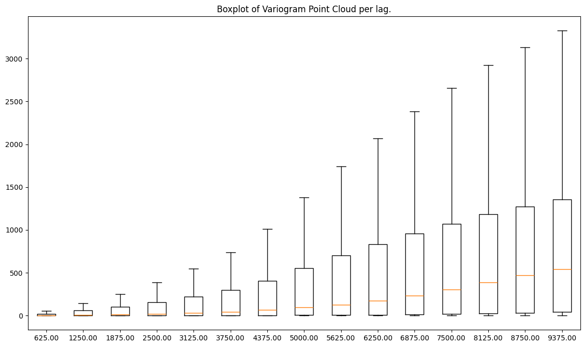
The orange line in the middle of each box represents the median (50%) value per lag. Now we can guess how the trend line goes, but, more importantly, we see other properties of semivariances within lags:
Dispersion of values is greater with a distance, but at the same time, median and the 3rd quartile of semivariance values are rising (3rd quartile is plotted as a horizontal line on a top of a box.
The maximum value rises with a distance (it is a horizontal line on a top of a whisker). Data is skewed towards lower values of semivariance. Why? Because the median is closer to the bottom of a box than the center or the top.
The 1st quartile (25% of the lowest values) is higher for distant lags.
Violin plot#
[8]:
vc.plot('violin');
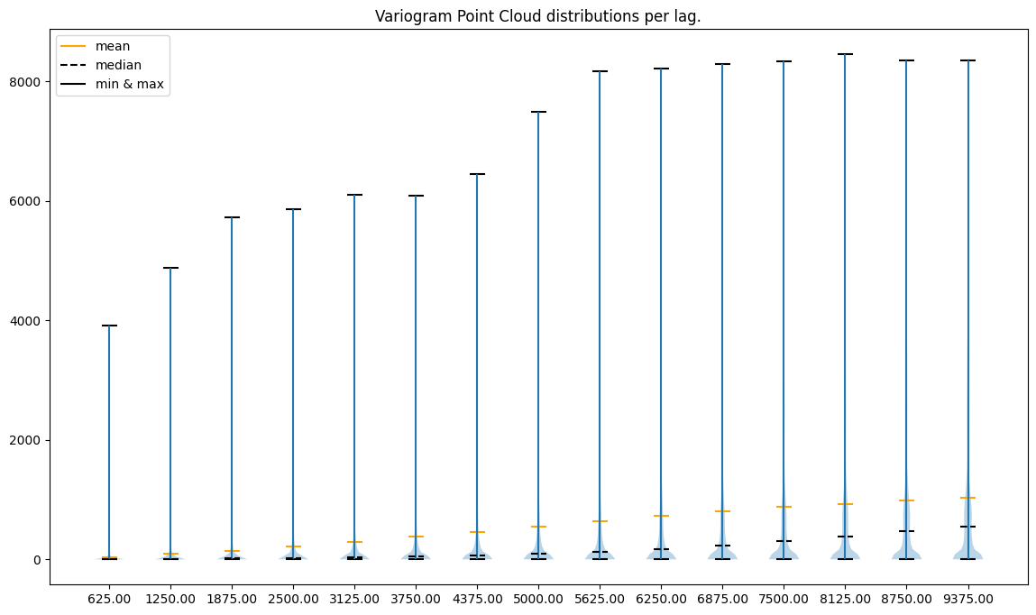
The violin plot supports our earlier assumptions, but we can find more insights here. For distant lags, distributions start to be multimodal. We see one mode around very low semivariance values and another close to the 1st quartile. Multimodality may affect our outcomes, and it may tell us that there is more than one level of spatial dependency.
3. Detect and remove outliers#
There is still the elephant in the room - box plot and violin plot show that data is skewed towards large semivariance values (long whiskers). Those outliers may affect later modeling, we should consider cleaning data before Kriging.
We can remove points with too low | too high DEM values, or we can remove anomalous semivariances from the point cloud.
Our data is skewed towards large values. Thus, we will remove outliers from the upper part of the distribution. We will use the interquartile range algorithm. It detects outliers as all points below the first quartile of a data plus m (positive or zero float) standard deviations and all points above the 3rd quartile plus n (positive or zero float) standard deviations. The important thing is that the absolute values of m and n can differ. We should fit those values to the
semivariance distributions.
The class VariogramCloud has internal method .remove_outliers(). With the parameter inplace set to True, we can overwrite the variogram point cloud, but if we set it to False, it will return the new VariogramCloud object with a cleaned variogram point cloud.
Other parameters that we are going to set of this method are:
method: We have two methods, one based on the z-score and the second based on the interquartile range. Both have upper and lower bounds. The Z-score method is invoked withmethod='zscore', and arguments for this function arez_lower_limitandz_upper_limit(number of standard deviations from the mean down and up, or negative and positive).iqr_lower_limit: how many standard deviations should be subtracted from the first quartile to set a limit of valid values,iqr_upper_limit: how many standard deviations should be added to the 3rd quartile to set a limit of valid values.
he values we will get will be within limits:
where:
\(q1\) - 1st quartile
\(q3\) - 3rd quartile
\(std\) - standard deviation
\(m\) - real number greater or equal than 0
\(n\) - real number greater or equal than 0
\(V\) - values in range
with the assumption, that \(q1\), \(q3\), \(std\), and \(V\) are lag-specific.
[9]:
cvc = vc.remove_outliers(
    method='iqr',
    iqr_lower_limit=4,
    iqr_upper_limit=1.5,
    inplace=False
)
[10]:
cvc.plot('box');
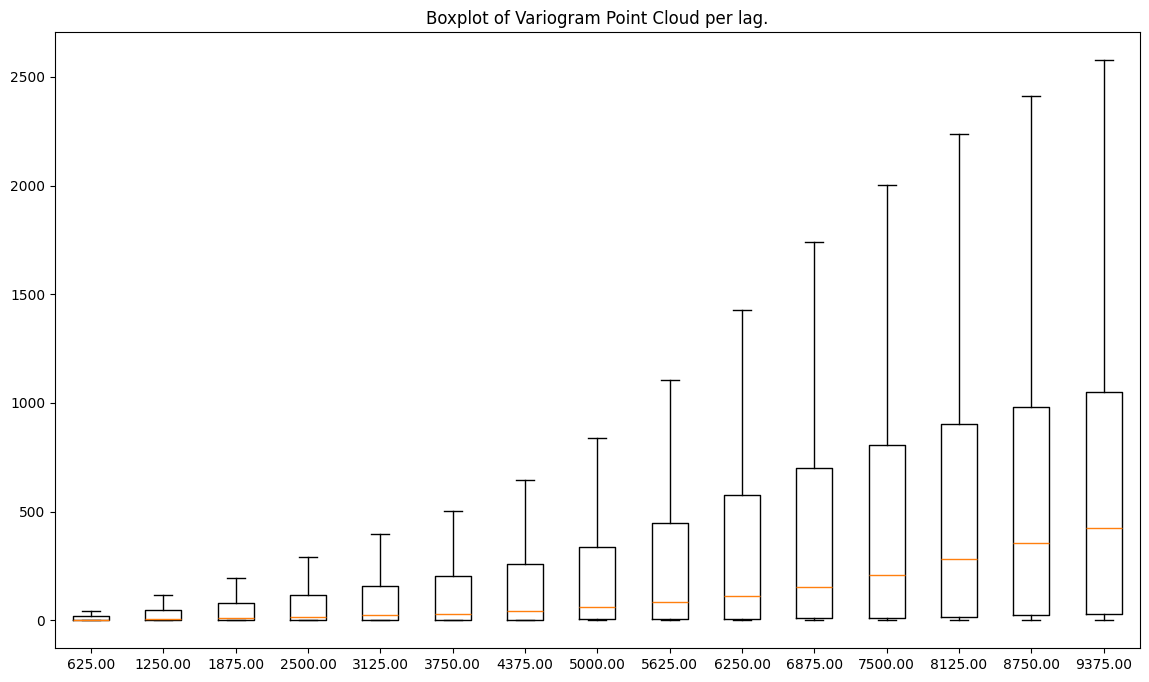
When we compare both figures - before and after data cleaning - we see that the y-axis of the second plot is few times smaller than the y-axis of the first plot! We’ve cleaned our data from the extreme values.
Note: removing outliers from semivariance is one way of dealing with non-normal data distributions, but you should proceed with caution when you remove your observations or derivatives from those observations. You should check tutorial
tutorials/functional/3-3-outliers-and-krigingto understand downsides of outliers removal.
4. Experimental variogram from the point cloud#
The last but not least property of the experimental variogram point cloud is that we may calculate the semivariogram directly from it using .calculate_experimental_variogram() method.
[11]:
exp_var = vc.experimental_semivariances()
[12]:
exp_var.plot(semivariance=True, covariance=False, variance=False)
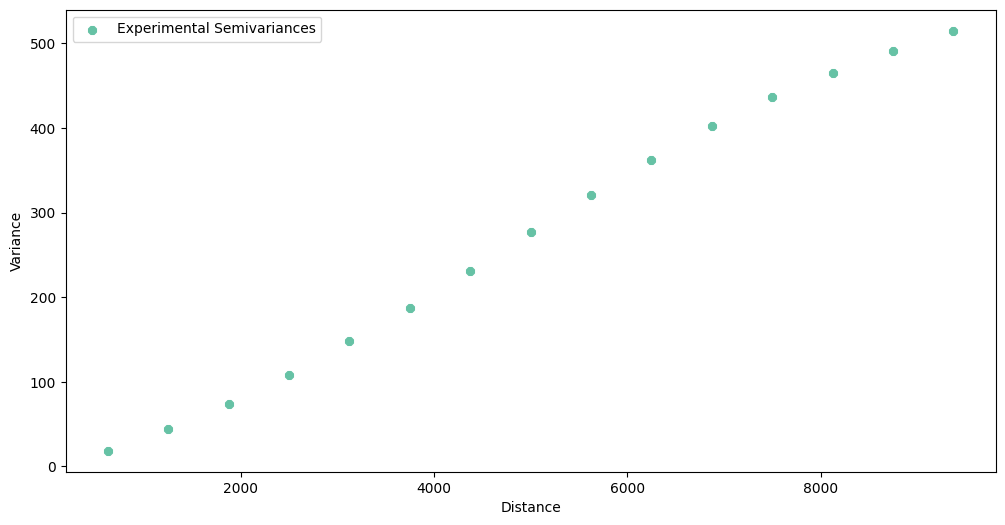
The same points are under mean row in .describe() method:
[13]:
vc.describe(as_dataframe=True).loc['mean']
[13]:
625.0      18.478983
1250.0     43.719468
1875.0     73.489310
2500.0    107.858598
3125.0    147.852660
3750.0    187.597718
4375.0    231.297386
5000.0    276.862155
5625.0    320.526495
6250.0    361.624234
6875.0    402.744376
7500.0    436.767505
8125.0    464.904780
8750.0    490.299066
9375.0    514.849220
Name: mean, dtype: float64
[14]:
exp_var.semivariances
[14]:
array([ 18.47898266,  43.71946771,  73.48930987, 107.8585979 ,
       147.85265986, 187.59771789, 231.29738612, 276.86215475,
       320.52649515, 361.62423403, 402.74437591, 436.76750526,
       464.90478027, 490.29906598, 514.84922016])
5. Is variogram point cloud a scatter plot?#
Yes, it is. But in pyinterpolate, we aggregated semivariances within bins (lags). If we remove bins (lags) completely then we get a scatter plot of semivariances. To simulate this behavior, we will create variogram cloud with 1000 lags.
[15]:
step_size = max_range / 1000
[16]:
vc1000 = VariogramCloud(
    values=dem['dem'],
    geometries=dem['geometry'],
    step_size=step_size,
    max_range=max_range
)
[17]:
vc1000.plot('scatter');
/Users/szymonos/Documents/GitHub/pyinterpolate/src/pyinterpolate/semivariogram/experimental/classes/variogram_cloud.py:545: RuntimeWarning: invalid value encountered in scalar divide
  bin_width = (no * max_width) / max_no

Changelog#
Date |
Changes |
Author |
|---|---|---|
2025-11-07 |
Used values and geometries parameters instead of ds in the experimental variogram initialization |
@SimonMolinsky (Szymon Moliński) |
2025-04-26 |
Tutorial has been adapted to the 1.0 release |
@SimonMolinsky (Szymon Moliński) |
[ ]: