Blocks to points with Ordinary Kriging#
This tutorial is based on the question of user @ikey from Discord channel of the package (02/04/2021). Thank you @ikey for your question!
Q:
Are we able to perform Semivariogram Regularization and Poisson Kriging if our point support represents only points without any values?
No, it’s not possible. But there is a hack that we can use - we can interpolate missing values from areal centroids with Ordinary and Simple Kriging just like we do with regular points. Why is this not possible with unknown points?
The idea behind semivariogram regularization of areal aggregates is to use semivariogram of point support. Point support must reflect an ongoing process. For example, in the case of epidemiology:
We have areal counts of infections divided by POPULATION over some areas (infection rates).
We take POPULATION blocks (points) with a number of inhabitants per block and use those as support for our map. Thus, we transform the choropleth map into the point map, taking only points where someone is living and might be infected. In other words, we use point values (population size) used in the denominator of the variable aggregated in choropleth map. We skip large parts of the map where the risk of infection is not present because no one is living there.
We obtain the population-at-risk map of points or smoothed choropleth map of infection risk without large visual bias where large/small areas seem to be more important, and infection risk is dispersed over the populated places.
This works when we have counted observations divided by another parameter (time, population, probability, volume, etc.). Without support values, e.g.: rate denominator, we are not able to perform semivariogram regularization.
What we want to achieve - transforming block data into point grid without any values - might be done using Ordinary Kriging, and semivariogram regularization is not required (and not possible when denominator is equal to zero).
In summary, this notebook shows how to transform blocks data into a pre-defined point grid, where points of the point grid don’t have any meaning.
Prerequisites#
Domain:
semivariance and covariance functions
kriging (basics)
outliers removal
Package:
ordinary_kriging()interpolate_points()VariogramCloud()
Programming:
Python basics
pandasbasics
Table of contents#
Prepare data
Detect and remove outliers
Fit semivariogram model
Prepare canvas
Interpolate from blocks on a given canvas
1. Prepare data#
The block data represents the breast cancer rates in the Northeastern part of the United States. Rate is the number of new cases divided by the population in a county, and this fraction is multiplied by a constant factor of 100,000.
[1]:
import numpy as np
import geopandas as gpd

import matplotlib.pyplot as plt
from pyinterpolate import Blocks, VariogramCloud, TheoreticalVariogram, interpolate_points
[2]:
DATASET = '../data/blocks/cancer_data.gpkg'
CANVAS = '../data/blocks/regular_grid_points.shp'

POLYGON_LAYER = 'areas'
GEOMETRY_COL = 'geometry'
POLYGON_ID = 'FIPS'
POLYGON_VALUE = 'rate'
[3]:
AREAL_INPUT = Blocks(
    ds=gpd.read_file(DATASET, layer=POLYGON_LAYER),
    value_column_name=POLYGON_VALUE,
    index_column_name=POLYGON_ID
)
AREAL_INPUT.ds.head()
[3]:
| FIPS | rate | geometry | representative_points | lon | lat | |
|---|---|---|---|---|---|---|
| 0 | 25019 | 192.2 | MULTIPOLYGON (((2115688.816 556471.24, 2115699... | POINT (2133348.745 558025.221) | 2.133349e+06 | 558025.221156 |
| 1 | 36121 | 166.8 | POLYGON ((1419423.43 564830.379, 1419729.721 5... | POINT (1442153.243 550673.936) | 1.442153e+06 | 550673.935704 |
| 2 | 33001 | 157.4 | MULTIPOLYGON (((1937530.728 779787.978, 193751... | POINT (1958207.252 766008.62) | 1.958207e+06 | 766008.620010 |
| 3 | 25007 | 156.7 | MULTIPOLYGON (((2074073.532 539159.504, 207411... | POINT (2084187.905 556436.412) | 2.084188e+06 | 556436.412055 |
| 4 | 25001 | 155.3 | MULTIPOLYGON (((2095343.207 637424.961, 209528... | POINT (2101100.939 600344.125) | 2.101101e+06 | 600344.124709 |
[4]:
areal_centroids = AREAL_INPUT.ds[['lon', 'lat', 'rate']].to_numpy()
areal_centroids[0]
[4]:
array([2.13334874e+06, 5.58025221e+05, 1.92200000e+02])
2. Detect and remove outliers#
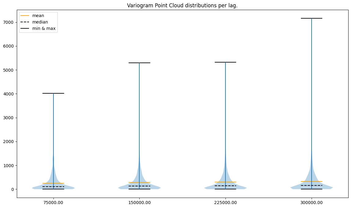
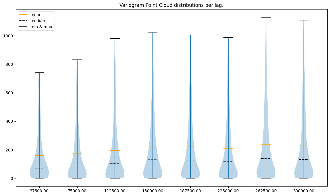
We will clean data before the semivariogram fitting and the Ordinary Kriging interpolation. Variogram Point Cloud is the best way to analyze data and detect outliers. We inspect |and compare different lags and step sizes and their respective point clouds. Then we will create multiple variograms and Kriging models.
[5]:
# Create analysis parameters

maximum_range = 300000

number_of_lags = [4, 8, 16]
step_sizes = [maximum_range / x for x in number_of_lags]

variogram_clouds = []

for step_size in step_sizes:
    max_range = maximum_range + step_size
    vc = VariogramCloud(values=areal_centroids[:, -1],
                        geometries=areal_centroids[:, :-1],
                        step_size=step_size,
                        max_range=max_range)
    variogram_clouds.append(vc)
[6]:
for vc in variogram_clouds:
    print(f'Lags per area: {len(vc.lags)}')
    print('')
    vc.plot('violin')
    print('\n###########\n')
Lags per area: 4
###########

Lags per area: 8
###########

Lags per area: 16
###########
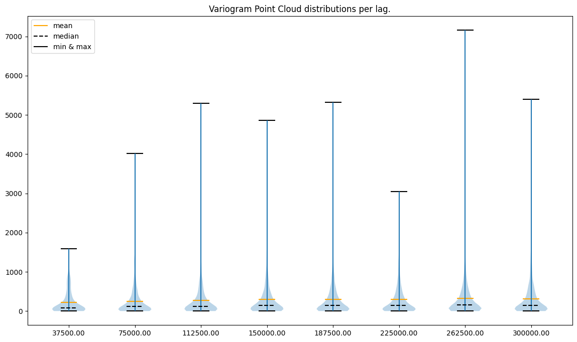
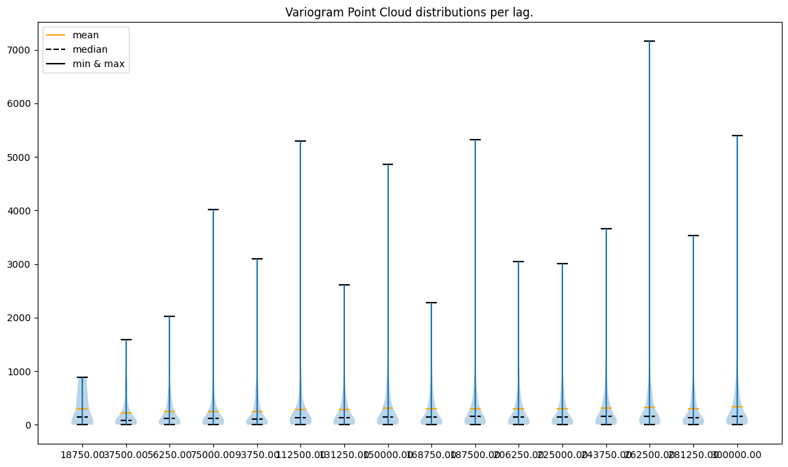
What do plots tell us?
point to point errors per lag are skewed toward positive values (the mean is always greater than the median)
less lags == less variability
variability in the last case (16 lags) seems to be too high
variability in the first case (4 lags) seems to be too small
there are extreme semivariance values, and the largest extremities are present for the most distant lags
What can we do?
remove outliers (extremely high semivariances) in each lag
use a small number of neighbors and a range close to 200,000 to avoid unnecessary computations
[7]:
# Now remove outliers from each lag

_ = [
    vc.remove_outliers(
        method='iqr',
        iqr_lower_limit=3,
        iqr_upper_limit=1.5,
        inplace=True
    ) for vc in variogram_clouds
]
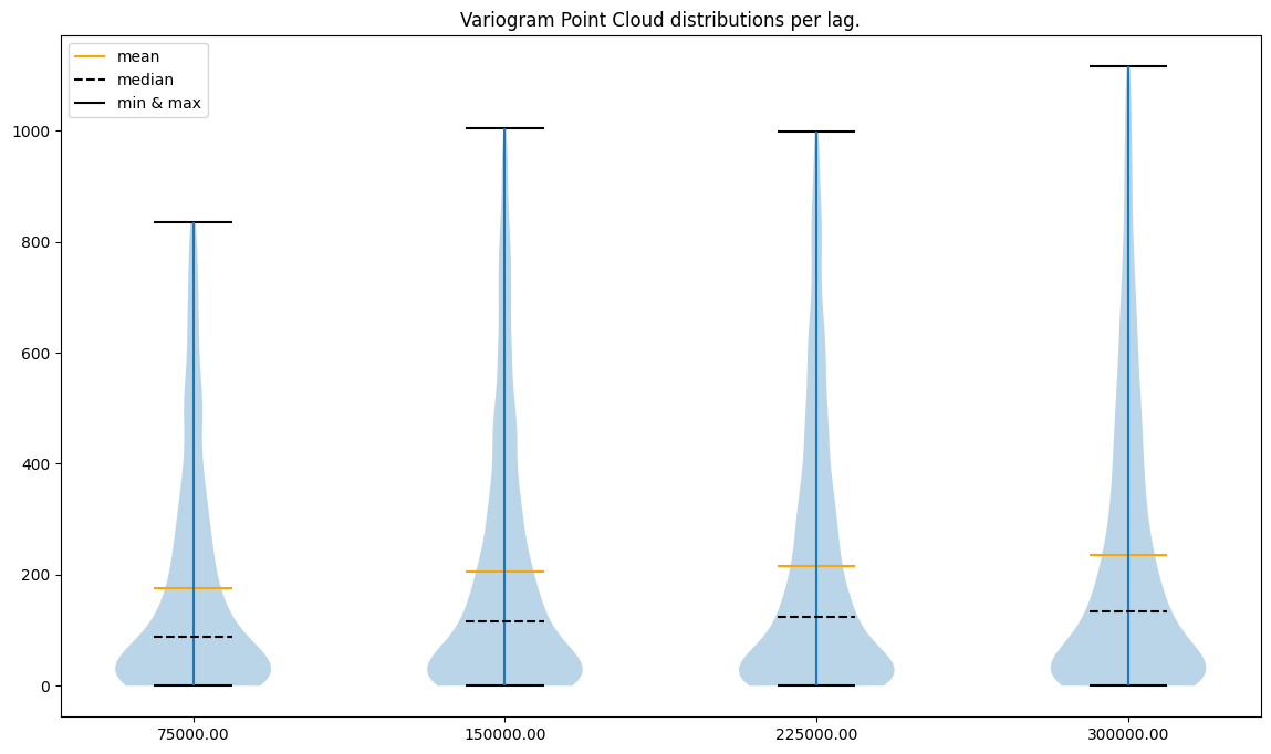
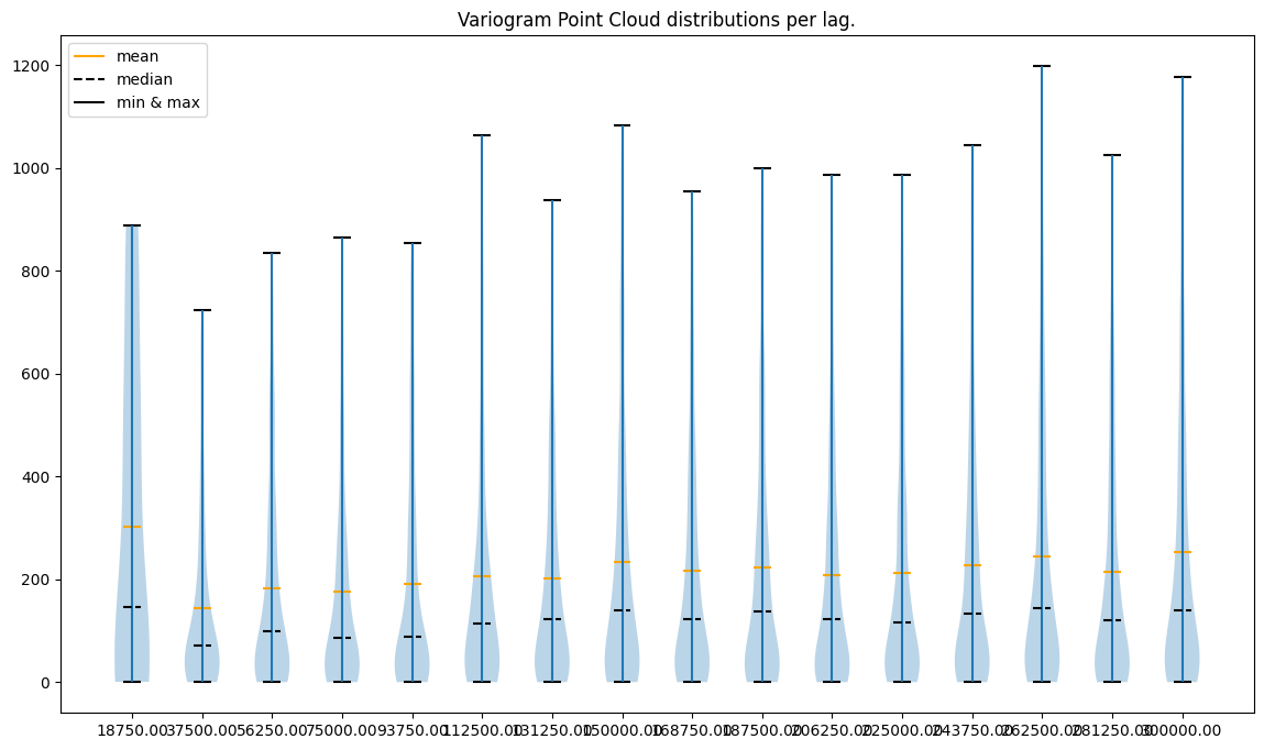
[8]:
# And show data without outliers

for vc in variogram_clouds:
    print(f'Lags per area: {len(vc.lags)}')
    print('')
    vc.plot('violin')
    print('\n###########\n')
Lags per area: 4
###########

Lags per area: 8
###########

Lags per area: 16
###########
If we compare the y axis before and after removing outliers, we may see that values are now smaller and densely populated. The variability for 16 lags, especially at the low ranges, is too high. Model build on top of this variogram might behave poorly.
3. Fit semivariogram model#
Semivariogram may be fitted manually or automatically. In this case, we fit it automatically - we test multiple models. We didn’t force any model to see how different results we would get.
[9]:
theoretical_semivariograms = []

for idx, vc in enumerate(variogram_clouds):

    print(f'Semivariance calculated for {len(vc.lags)} lags.')

    # Calculate experimental model
    exp_model = vc.experimental_semivariances()

    # Assign experimental model and data to TheoreticalSemivariogram
    theo_semi = TheoreticalVariogram()
    theo_semi.autofit(experimental_variogram=exp_model)
    theoretical_semivariograms.append(theo_semi)
    print('')
    print('Model parameters:')
    print('Model type:', theo_semi.name)
    print('Nugget:', theo_semi.nugget)
    print('Sill:', theo_semi.sill)
    print('Range:', theo_semi.rang)
    print('Model error:', theo_semi.rmse)
    print('')
    print('')
Semivariance calculated for 4 lags.

Model parameters:
Model type: spherical
Nugget: 36.47814412070759
Sill: 113.9843806262891
Range: 130635.90676540829
Model error: 6.013657676895086


Semivariance calculated for 8 lags.

Model parameters:
Model type: spherical
Nugget: 56.468678977272724
Sill: 91.20165827269054
Range: 130635.90676540829
Model error: 9.285171141696564


Semivariance calculated for 16 lags.

Model parameters:
Model type: spherical
Nugget: 75.54535714285717
Sill: 78.23809400314832
Range: 165472.14856951716
Model error: 17.306288625624866
Each case has a different model type, a different sill, and a different range! How do we choose the model parameters appropriately in this scenario? Error rises with the number of lags but is it a good indicator of the semivariogram fit? No, and we should be careful when choosing variograms with a few lags instead of variograms with multiple lags. We may miss some spatial patterns that will be averaged with a smaller number of lags. We will choose variogram with 8 lags, even if the error is not the best.
4. Prepare canvas#
Our variogram model is ready to load the point file as the GeoDataFrame object, which stores the geometry column and data features as tables.
[10]:
gdf_pts = gpd.read_file(CANVAS)
gdf_pts.crs == AREAL_INPUT.ds.crs
[10]:
True
[11]:
gdf_pts.set_index('id', inplace=True)
gdf_pts['x'] = gdf_pts.geometry.x
gdf_pts['y'] = gdf_pts.geometry.y
gdf_pts.head()
[11]:
| geometry | x | y | |
|---|---|---|---|
| id | |||
| 81.0 | POINT (1277277.671 441124.507) | 1.277278e+06 | 441124.5068 |
| 82.0 | POINT (1277277.671 431124.507) | 1.277278e+06 | 431124.5068 |
| 83.0 | POINT (1277277.671 421124.507) | 1.277278e+06 | 421124.5068 |
| 84.0 | POINT (1277277.671 411124.507) | 1.277278e+06 | 411124.5068 |
| 85.0 | POINT (1277277.671 401124.507) | 1.277278e+06 | 401124.5068 |
5. Interpolate#
We can model all values in a batch using function interpolate_points().
Based on the learning from a semivariogram modeling step, we will set a number of neighboring areas to 8 and range to 200000. We will append interpolated values and errors to an existing data frame and plot them to compare results.
[12]:
preds_cols = []
errs_cols = []

for semi_model in theoretical_semivariograms:
    kriged = interpolate_points(
        theoretical_model=semi_model,
        known_values=areal_centroids[:, -1],
        known_geometries=areal_centroids[:, :-1],
        unknown_locations=gdf_pts[['x', 'y']].to_numpy(),
        neighbors_range=200000,
        no_neighbors=16,
        use_all_neighbors_in_range=True
    )

    # Interpolate missing values and uncertainty
    pred_col_name = 'p ' + semi_model.name[:3] + ' ' + str(len(semi_model.lags))
    uncertainty_col_name = 'e ' + semi_model.name[:3] + ' ' + str(len(semi_model.lags))
    gdf_pts[pred_col_name] = kriged[:, 0]
    gdf_pts[uncertainty_col_name] = kriged[:, 1]
    preds_cols.append(pred_col_name)
    errs_cols.append(uncertainty_col_name)
100%|██████████| 5419/5419 [01:02<00:00, 86.91it/s]
100%|██████████| 5419/5419 [00:18<00:00, 285.90it/s]
100%|██████████| 5419/5419 [00:02<00:00, 2350.68it/s]
[13]:
gdf_pts.head()
[13]:
| geometry | x | y | p sph 4 | e sph 4 | p sph 8 | e sph 8 | p sph 16 | e sph 16 | |
|---|---|---|---|---|---|---|---|---|---|
| id | |||||||||
| 81.0 | POINT (1277277.671 441124.507) | 1.277278e+06 | 441124.5068 | 131.300950 | 102.178639 | 131.300950 | 109.037233 | 133.190048 | 112.323151 |
| 82.0 | POINT (1277277.671 431124.507) | 1.277278e+06 | 431124.5068 | 129.939483 | 100.512382 | 129.939483 | 107.704020 | 130.831391 | 111.218534 |
| 83.0 | POINT (1277277.671 421124.507) | 1.277278e+06 | 421124.5068 | 129.052488 | 99.533481 | 129.052488 | 106.920779 | 129.964626 | 110.470425 |
| 84.0 | POINT (1277277.671 411124.507) | 1.277278e+06 | 411124.5068 | 128.396747 | 98.920356 | 128.396747 | 106.430202 | 129.282825 | 110.013474 |
| 85.0 | POINT (1277277.671 401124.507) | 1.277278e+06 | 401124.5068 | 128.288679 | 98.517309 | 128.288679 | 106.107714 | 129.215478 | 109.573660 |
Now we can save our GeoDataFrame as a geopackage or proceed with the analysis.
[14]:
# Save interpolation results

# gdf_pts.to_file('interpolation_results_areal_to_point.gpkg')
[15]:
# Now compare results to choropleth maps
fig, axes = plt.subplots(nrows=2, ncols=3, figsize=(16, 16), sharex='all', sharey='all')

base1 = AREAL_INPUT.ds.plot(ax=axes[0, 0], legend=True, edgecolor='black', color='white')
base2 = AREAL_INPUT.ds.plot(ax=axes[0, 1], legend=True, edgecolor='black', color='white')
base3 = AREAL_INPUT.ds.plot(ax=axes[0, 2], legend=True, edgecolor='black', color='white')
base4 = AREAL_INPUT.ds.plot(ax=axes[1, 0], legend=True, edgecolor='black', color='white')
base5 = AREAL_INPUT.ds.plot(ax=axes[1, 1], legend=True, edgecolor='black', color='white')
base6 = AREAL_INPUT.ds.plot(ax=axes[1, 2], legend=True, edgecolor='black', color='white')

gdf_pts.plot(ax=base1, column=preds_cols[0], cmap='Spectral_r', alpha=0.3)
gdf_pts.plot(ax=base2, column=preds_cols[1], cmap='Spectral_r', alpha=0.3)
gdf_pts.plot(ax=base3, column=preds_cols[2], cmap='Spectral_r', alpha=0.3)
gdf_pts.plot(ax=base4, column=errs_cols[0], cmap='Reds', alpha=0.3)
gdf_pts.plot(ax=base5, column=errs_cols[1], cmap='Reds', alpha=0.3)
gdf_pts.plot(ax=base6, column=errs_cols[2], cmap='Reds', alpha=0.3)

axes[0, 0].set_title(preds_cols[0])
axes[0, 1].set_title(preds_cols[1])
axes[0, 2].set_title(preds_cols[2])
axes[1, 0].set_title(errs_cols[0])
axes[1, 1].set_title(errs_cols[1])
axes[1, 2].set_title(errs_cols[2])

plt.suptitle('Comparison of different Kriging models outputs')
plt.show()
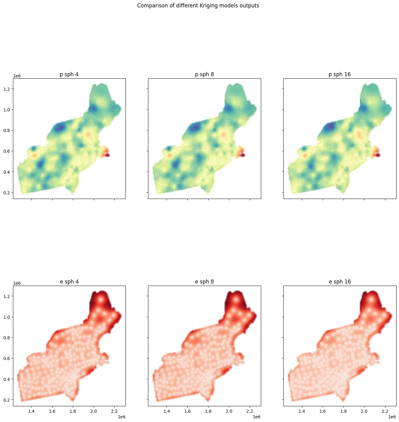
Are absolute errors between maps large or not? Let’s check it in the last step:
[16]:
for pcol1 in preds_cols:
    print('Column:', pcol1)
    for pcol2 in preds_cols:
        if pcol1 == pcol2:
            pass
        else:
            mad = gdf_pts[pcol1] - gdf_pts[pcol2]
            mad = np.abs(np.mean(mad))
            print(f'Mean Absolute Difference with {pcol2} is {mad:.9f}')
    print('')
Column: p sph 4
Mean Absolute Difference with p sph 8 is 0.000000000
Mean Absolute Difference with p sph 16 is 0.020515483

Column: p sph 8
Mean Absolute Difference with p sph 4 is 0.000000000
Mean Absolute Difference with p sph 16 is 0.020515483

Column: p sph 16
Mean Absolute Difference with p sph 4 is 0.020515483
Mean Absolute Difference with p sph 8 is 0.020515483
Model with 4 lags and model with 8 lags give almost the same results because range of both models is very close.
Changelog#
Date |
Changes |
Author |
|---|---|---|
2025-11-07 |
Used values and geometries parameters instead of ds in the experimental variogram initialization, and known_values and known_geometries for kriging process (instead of known_locations parameter) |
@SimonMolinsky (Szymon Moliński) |
2025-05-18 |
Tutorial has been adapted to the 1.0 release |
@SimonMolinsky (Szymon Moliński) |