Directional Ordinary Kriging#
In this tutorial, we will learn about Ordinary Kriging using a directional semivariogram. The classic Kriging works with an isotropic semivariogram. Actual geographical data is rarely isotropic, and we may distinguish leading direction of a process. The example may be a temperature, where differences in the North-South axis are greater than in the West-East axis.
Prerequisites#
Domain:
semivariance and covariance functions
kriging (basics)
directional semivariogram
Package:
DirectionalVariogram()interpolate_points()
Programming:
Python basics
pandasbasics
Table of contents#
Prepare data
Create directional semivariograms
Interpolate with directional Kriging
Compare results
Prepare data#
We use meuse dataset and interpolate zinc concentrations. Dataset is provided in: Pebesma, Edzer. (2009). The meuse data set: a tutorial for the gstat R package
[1]:
import geopandas as gpd
import numpy as np
import pandas as pd

import matplotlib.pyplot as plt

from pyinterpolate import DirectionalVariogram, TheoreticalVariogram, \
    interpolate_points
[2]:
MEUSE_FILE = '../data/meuse/meuse.csv'
MEUSE_GRID_FILE = '../data/meuse/meuse_grid.csv'
[3]:
# Variogram parameters
STEP_SIZE = 100
MAX_RANGE = 1600
[4]:
df = pd.read_csv(MEUSE_FILE, usecols=['x', 'y', 'zinc'])
[5]:
df.head()
[5]:
| x | y | zinc | |
|---|---|---|---|
| 0 | 181072 | 333611 | 1022 |
| 1 | 181025 | 333558 | 1141 |
| 2 | 181165 | 333537 | 640 |
| 3 | 181298 | 333484 | 257 |
| 4 | 181307 | 333330 | 269 |
[6]:
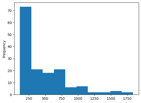
# Distribution

df['zinc'].plot(kind='hist')
[6]:
<Axes: ylabel='Frequency'>
[7]:
df['log-zinc'] = np.log(df['zinc'])
[8]:
df['log-zinc'].plot(kind='hist')
[8]:
<Axes: ylabel='Frequency'>
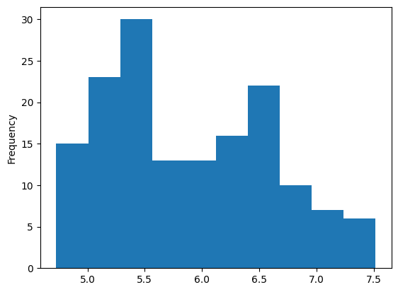
The histogram is still not close to the normal distribution; it has two modes, but the tail is shorter. We will build models based on this histogram.
2. Create directional semivariograms#
Data is prepared, we can model it’s semivariance. We will perform an isotropic modeling and a full directional modeling in N-S, W-E, NE-SW, and NW-SE axes.
[9]:
dirvar = DirectionalVariogram(values=df['log-zinc'],
                              geometries=df[['x', 'y']],
                              step_size=STEP_SIZE,
                              max_range=MAX_RANGE,
                              tolerance=0.5)
dirvar.show()
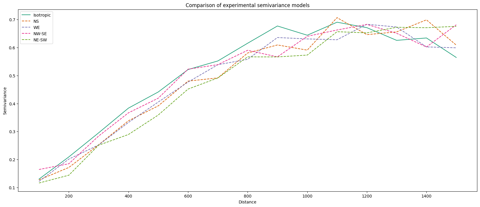
We have five experimental variograms for further modeling. Let’s build theoretical models from those.
[10]:
MODEL_NAME = 'spherical'
DIRECTIONS = ['ISO', 'NS', 'WE', 'NE-SW', 'NW-SE']
[11]:
theoretical_models = {}
variograms = dirvar.get()

for direction in DIRECTIONS:
    theoretical_model = TheoreticalVariogram()
    theoretical_model.autofit(experimental_variogram=variograms[direction],
                              models_group=MODEL_NAME,
                              nugget=0)
    theoretical_models[direction] = theoretical_model
3. Interpolate with directional Kriging#
With a set of directional variograms we will perform spatial interpolation over a defined grid.
[12]:
grid = pd.read_csv(MEUSE_GRID_FILE, usecols=['x', 'y'])
grid.head()
[12]:
| x | y | |
|---|---|---|
| 0 | 181180 | 333740 |
| 1 | 181140 | 333700 |
| 2 | 181180 | 333700 |
| 3 | 181220 | 333700 |
| 4 | 181100 | 333660 |
[13]:
kriged_results = {}

for direction in DIRECTIONS:
    result = interpolate_points(
        theoretical_model=theoretical_models[direction],
        known_values=df['log-zinc'],
        known_geometries=df[['x', 'y']],
        unknown_locations=grid.to_numpy(),
        no_neighbors=16,
        max_tick=30,
        use_all_neighbors_in_range=False
    )
    result = pd.DataFrame(result, columns=['pred', 'err', 'x', 'y'])
    rgeometry = gpd.points_from_xy(result['x'], result['y'])
    rgeometry.name = 'geometry'
    result = gpd.GeoDataFrame(result, geometry=rgeometry)

    kriged_results[direction] = result
100%|██████████| 3103/3103 [00:03<00:00, 888.74it/s]
100%|██████████| 3103/3103 [00:07<00:00, 441.79it/s]
100%|██████████| 3103/3103 [00:05<00:00, 518.33it/s]
100%|██████████| 3103/3103 [00:05<00:00, 550.24it/s]
100%|██████████| 3103/3103 [00:06<00:00, 464.40it/s]
[14]:
kriged_results['ISO'].head()
[14]:
| pred | err | x | y | geometry | |
|---|---|---|---|---|---|
| 0 | 6.614562 | 0.270738 | 181180.0 | 333740.0 | POINT (181180 333740) |
| 1 | 6.717101 | 0.187153 | 181140.0 | 333700.0 | POINT (181140 333700) |
| 2 | 6.594676 | 0.212485 | 181180.0 | 333700.0 | POINT (181180 333700) |
| 3 | 6.471774 | 0.239660 | 181220.0 | 333700.0 | POINT (181220 333700) |
| 4 | 6.838043 | 0.100923 | 181100.0 | 333660.0 | POINT (181100 333660) |
With all models calculated, we can compare the results of interpolation. We will show interpolation and variance errors across the models.
4. Compare models#
[15]:
fig, ax = plt.subplots(nrows=5, ncols=2, figsize=(15, 20))

kriged_results['ISO'].plot(ax=ax[0, 0], column='pred', cmap='cividis', s=0.25)
kriged_results['ISO'].plot(ax=ax[0, 1], column='err', cmap='Reds', s=0.25)
ax[0, 0].set_title('Prediction - isotropic')
ax[0, 1].set_title('Error - isotropic')

kriged_results['NS'].plot(ax=ax[1, 0], column='pred', cmap='cividis', s=0.25)
kriged_results['NS'].plot(ax=ax[1, 1], column='err', cmap='Reds', s=0.25)
ax[1, 0].set_title('Prediction - NS')
ax[1, 1].set_title('Error - NS')

kriged_results['WE'].plot(ax=ax[2, 0], column='pred', cmap='cividis', s=0.25)
kriged_results['WE'].plot(ax=ax[2, 1], column='err', cmap='Reds', s=0.25)
ax[2, 0].set_title('Prediction - WE')
ax[2, 1].set_title('Error - WE')

kriged_results['NE-SW'].plot(ax=ax[3, 0], column='pred', cmap='cividis', s=0.25)
kriged_results['NE-SW'].plot(ax=ax[3, 1], column='err', cmap='Reds', s=0.25)
ax[3, 0].set_title('Prediction - NE-SW')
ax[3, 1].set_title('Error - NE-SW')

kriged_results['NW-SE'].plot(ax=ax[4, 0], column='pred', cmap='cividis', s=0.25)
kriged_results['NW-SE'].plot(ax=ax[4, 1], column='err', cmap='Reds', s=0.25)
ax[4, 0].set_title('Prediction - NW-SE')
ax[4, 1].set_title('Error - NW-SE')

plt.show()
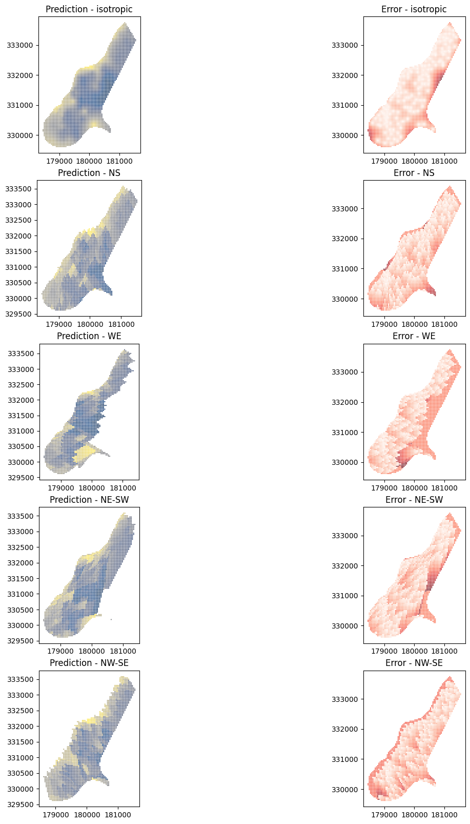
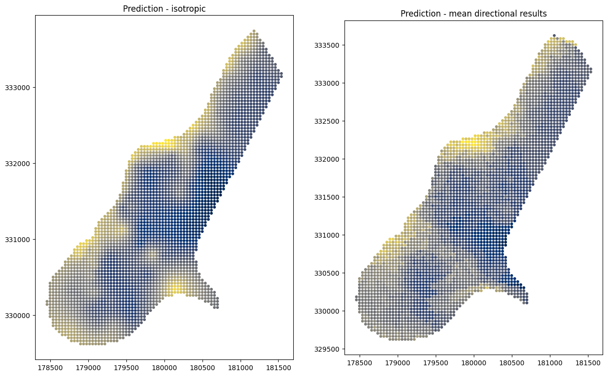
Directional Kriging clearly shows the leading direction and is even more pronounced in the variance error maps. At the end, let’s compare the mean of directional interpolations to the isotropic interpolation result:
[16]:
mean_directional_results = np.nanmean(
    np.array([
        kriged_results['NS']['pred'],
        kriged_results['WE']['pred'],
        kriged_results['NE-SW']['pred'],
        kriged_results['NW-SE']['pred']
    ]), axis=0
)
/var/folders/vv/zx11_2ts7tjfsny482gs54s80000gr/T/ipykernel_42139/81901919.py:1: RuntimeWarning: Mean of empty slice
  mean_directional_results = np.nanmean(
[17]:
kriged_results['ISO']['mean_dir_pred'] = mean_directional_results
[18]:
_, ax = plt.subplots(nrows=1, ncols=2, figsize=(15, 20))

kriged_results['ISO'].plot(ax=ax[0], column='pred', cmap='cividis', s=10)
ax[0].set_title('Prediction - isotropic')
kriged_results['ISO'].plot(ax=ax[1], column='mean_dir_pred', cmap='cividis', s=10)
ax[1].set_title('Prediction - mean directional results')
plt.show()
Changelog#
Date |
Changes |
Author |
|---|---|---|
2025-11-07 |
Used values and geometries parameters instead of ds in the experimental variogram initialization, and known_values and known_geometries for kriging process (instead of known_locations parameter) |
@SimonMolinsky (Szymon Moliński) |
2025-09-16 |
Removed |
@SimonMolinsky (Szymon Moliński) |
2025-05-17 |
Tutorial has been adapted to the 1.0 release |
@SimonMolinsky (Szymon Moliński) |