Benchmarking Kriging#
In this tutorial, we will learn how to validate our Kriging model. We’ll compare it to the Inverse Distance Weighting function, where the unknown point value is interpolated as the weighted mean of its neighbors. Weights are inversely proportional to the distance between neighboring points, decreasing faster when we raise denominator to the higher number.
Prerequisites#
Domain:
semivariance and covariance functions
kriging (basics)
Package:
TheoreticalVariogramExperimentalVariogramordinary_kriging()
Programming:
Python basics
pandasbasics
Table of contents#
Introduction - IDW as benchmarking tool.
Perform IDW and validate outputs.
Perform Kriging and validate outputs.
1. Introduction - IDW as bechmarking tool#
General Form of Inverse Distance Weighting
where:
\(z(u)\): predicted value
\(i\): i-th known location
\(z_{i}\): value at known location \(i\)
\(\lambda_{i}\): weight assigned to the point in known location \(i\)
Weighting Parameter
where:
\(d\): is a distance from the known point \(z_{i}\) to the unknown point \(z(u)\)
\(p\): is a hyperparameter that controls correlation between a known and unknown point. Greater \(p\) means that the influence of the closest neighbors is extremely high, but it quickly diminishes with a distance. On the other hand, you may set a small \(p\) to emphasize that even distant neighbors are influencing the unknown location.
IDW is a simple yet powerful technique. Unfortunately, it has a significant drawback: we must set \(p\) - power - manually, and it is constant across all distances. That’s why Kriging - in most cases - performs much better than IDW, weights are related to the distance to a neighbor, and are estimated when we build semivariogram model.
[1]:
import geopandas as gpd
import numpy as np
import pandas as pd

from tqdm import tqdm

from pyinterpolate import inverse_distance_weighting
from pyinterpolate import build_experimental_variogram, build_theoretical_variogram
from pyinterpolate import ordinary_kriging
[2]:
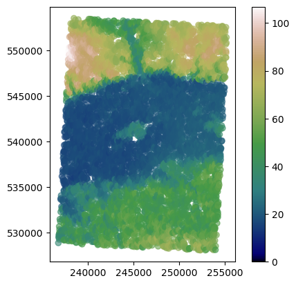
# Load DEM data

df = pd.read_csv(
    '../data/dem.csv'
)
# Populate geometry column and set CRS

dem_geometry = gpd.points_from_xy(x=df['longitude'], y=df['latitude'], crs='epsg:4326')
dem = gpd.GeoDataFrame(df, geometry=dem_geometry)

# Transform crs to metric values
dem.to_crs(epsg=2180, inplace=True)
dem.plot(column='dem', cmap='gist_earth', alpha=0.6, vmin=0, legend=True);
[3]:
step_size = 500  # meters
max_range = 10000  # meters
[4]:
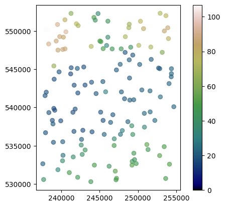
train = dem.sample(n=int(0.02*len(dem)))
test = dem.loc[~dem.index.isin(train.index)]
[5]:
print(len(train), len(test))
137 6758
[6]:
train.plot(column='dem', cmap='gist_earth', alpha=0.6, vmin=0, legend=True)
[6]:
<Axes: >
2. Perform IDW and validate outputs#
Inverse Distance Weighting doesn’t require variogram modeling. We pass the power parameter that affects weighting”. Things to remember are:”
large
powervalue -> closer neighbors are more importantpowerwhich is close to the zero -> all neighbors are important, and we assume that the distant process has the same effect on our variable as the closest neighbors
[7]:
idw_power = 2
number_of_neighbors = 8

idw_preds = test['geometry'].apply(
            lambda loc: inverse_distance_weighting(
                unknown_location=(loc.x, loc.y),
                known_values=train['dem'],
                known_geometries=train['geometry'],
                no_neighbors=number_of_neighbors,
                power=idw_power
            )
        )
[8]:
idw_rmse = np.mean(
    np.sqrt(
        (test['dem'] - idw_preds)**2
    )
)

print(f'Root Mean Squared Error of prediction with IDW is {idw_rmse}')
Root Mean Squared Error of prediction with IDW is 4.742992331513811
Clarification: Obtained Root Mean Squared Error could serve as a baseline for further model development. To build a better reference, we create four IDW models of powers:
0.5124
[9]:
IDW_POWERS = [0.5, 1, 4]  # we have 2 already
idws = {
    2: idw_rmse
}

for pw in tqdm(IDW_POWERS):
    idw_preds = test['geometry'].apply(
            lambda loc: inverse_distance_weighting(
                unknown_location=(loc.x, loc.y),
                known_values=train['dem'],
                known_geometries=train['geometry'],
                no_neighbors=number_of_neighbors,
                power=pw
            )
        )
    idw_rmse = np.mean(
        np.sqrt(
            (test['dem'] - idw_preds)**2
        )
    )
    idws[pw] = idw_rmse
100%|██████████| 3/3 [00:50<00:00, 16.88s/it]
[10]:
for pw, val in idws.items():
    print(f'Root Mean Squared Error of prediction with IDW of power {pw} is {val:.4f}')
Root Mean Squared Error of prediction with IDW of power 2 is 4.7430
Root Mean Squared Error of prediction with IDW of power 0.5 is 5.5618
Root Mean Squared Error of prediction with IDW of power 1 is 5.1866
Root Mean Squared Error of prediction with IDW of power 4 is 4.6035
3. Perform Kriging and validate outputs#
Now, we are going to compare IDW results to Kriging output.
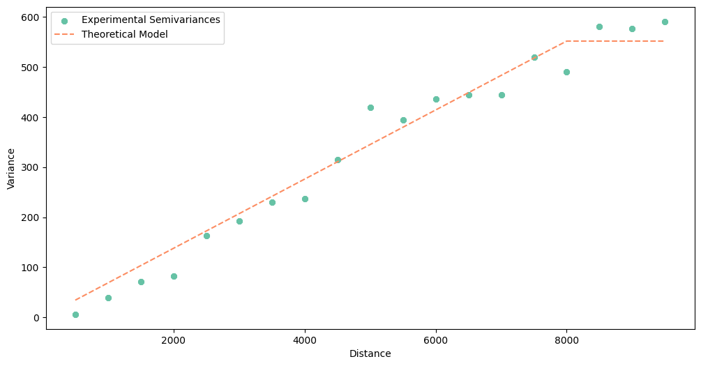
[11]:
exp_var = build_experimental_variogram(
    values=train['dem'],
    geometries=train['geometry'],
    step_size=step_size,
    max_range=max_range
)
[12]:
theo_var = build_theoretical_variogram(
    experimental_variogram=exp_var,
    models_group='linear'
)
[13]:
theo_var.plot()
[14]:
kriging_preds = ordinary_kriging(
    theoretical_model=theo_var,
    known_values=train['dem'],
    known_geometries=train['geometry'],
    unknown_locations=test['geometry'],
    no_neighbors=number_of_neighbors,
    allow_approximate_solutions=False)

kriging_preds = kriging_preds[:, 0]
100%|██████████| 6758/6758 [00:01<00:00, 4889.41it/s]
[15]:
kriging_rmse = np.mean(
    np.sqrt(
        (test['dem'] - kriging_preds)**2
    )
)
[16]:
print(f'Root Mean Squared Error of prediction with Kriging is {kriging_rmse}')
Root Mean Squared Error of prediction with Kriging is 4.583546966509806
Your results may be different (if your train and test sets are divided in a different way), but in most cases, Kriging will be better than IDW or very close to the best results from IDW. Even more important is that for the single data source with a low number of samples, we don’t have the opportunity to perform the validation step, and we’re unable to guess how big the power parameter should be. With Kriging, we model variogram, and voila! - model works.
Changelog#
Date |
Changes |
Author |
|---|---|---|
2025-11-07 |
Used values and geometries parameters instead of ds in the experimental variogram initialization, and known_values and known_geometries for kriging process (instead of known_locations parameter), the same for |
@SimonMolinsky (Szymon Moliński) |
2025-05-02 |
Tutorial has been adapted to the 1.0 release |
@SimonMolinsky (Szymon Moliński) |
2025-07-11 |
Changed behavior of |
@SimonMolinsky (Szymon Moliński) |
[ ]: